
USING LOGARITHMIC OPINION POOLING TECHNIQUES IN
BAYESIAN BLIND MULTI-CHANNEL RESTORATION
Bruno Amizic, Aggelos K. Katsaggelos
Department of Electrical Engineering and Computer Sciance, Northwestern University, 2145 Sheridan Rd, Evanston, USA
Rafael Molina
Departamento de Ciencias de la Computaci´on e I.A., Universidad de Granada, 18071 Granada, Spain
Keywords:
Bayesian framework, blind multi-channel restoration, logarithmic opinion pooling, variational methods.
Abstract:
In this paper we examine the use of logarithmic opinion pooling techniques to combine two observations mod-
els that are normally used in multi-channel image restoration techniques. The combined observation model is
used together with simultaneous autoregression prior models for the image and blurs to define the joint distri-
bution of image, blurs and observations. Assuming that all the unknown parameters are previously estimated
we use variational techniques to approximate the posterior distribution of the real underlying image and the
unknown blurs. We will examine the use of two approximations of the posterior distribution. Experimental
results are used to validate the proposed approach.
1 INTRODUCTION
Blind image restoration (BIR) has been an active re-
search topic for many years now (for the recent lit-
erature review see (Bishop et al., 2007)). In the BIR
solutions (Molina et al., 2006) both the original im-
age and blur are considered to be unknown. Blind
multi-channel restoration (BMCR) is an extension to
the BIR problem when multiple views of the scene are
available. Both BIR and BMCR are ill-possed prob-
lems. There are numerous practical applications in
which BMCR can be used. Satellite imaging, remote
sensing, astronomical imaging, microscopy and video
processing are some of the applications where multi-
ple distorted views of the original scene are available.
In this paper we propose solutions to the BMCR
problem based on the Bayesian paradigm, which
has already been widely used for image restoration
(Molina et al., 1999), (Mateos et al., 2000), (Galat-
sanos et al., 2002), removal of blocking artifacts (Ma-
teos et al., 2000) and deconvolution with partially
known blurs (Galatsanos et al., 2002).
For our BMCR problem formulation it is assumed
that L distorted versions of the original scene are
available. Each observation is modeled by a Linear
Space Invariant (LSI) system. Therefore, the output g
i
for each individual channel is given in vector-matrix
form by
g
i
= H
i
f+ n
i
, i = 1, 2,...,L, (1)
where f is the original image, n
i
represents the addi-
tive noise per channel, and H
i
represents the unknown
blur matrix which is approximated by an N×N block-
circulant matrix (all vectors are of size N × 1). It
should be pointed out that for the observations that
are not spatially aligned, matrix H
i
will also be used
to model any possible spatial shift. Before we proceed
further, let us rewrite Equation 1 in a more compact
form as
g = Hf+ n = Fh+ n, (2)
where g =
g
T
1
,g
T
2
,...,g
T
L
T
, h =
h
T
1
,h
T
2
,...,h
T
L
T
,
H =
H
T
1
,H
T
2
,...,H
T
L
T
, and n =
n
T
1
,n
T
2
,...,n
T
L
T
. Ma-
trix F has size LN× N and represents the block diag-
onal convolutional matrix.
In this work, our goal is to formulate the BMCR
problem by constructively combining different obser-
vations models and to use the variational approach
to approximate the joint posterior distribution of the
original image and blurs given the multi-channel ob-
servations.
This paper is organized as follows. In Section
2, we examine the Bayesian modeling of the multi-
channel restoration problem which allows us to com-
bine different observation models. In Section 3 we
565
Amizic B., K. Katsaggelos A. and Molina R. (2008).
USING LOGARITHMIC OPINION POOLING TECHNIQUES IN BAYESIAN BLIND MULTI-CHANNEL RESTORATION.
In Proceedings of the Third International Conference on Computer Vision Theory and Applications, pages 565-570
DOI: 10.5220/0001091405650570
Copyright
c
SciTePress

use variational techniques to approximate the joint
posterior distribution of the original image and blurs
given the multi-channel observations. In Section 4 we
present experimental results and present the conclu-
sions in Section 5.
2 BAYESIAN FRAMEWORK
On the unknown image we assume that its luminos-
ity distribution is smooth, and therefore we choose
the simultaneous autoregression (SAR) model (Rip-
ley, 1981) as the image prior,
p(f | α
im
) ∝ exp
−
1
2
α
im
kCfk
2
. (3)
Matrix C has size N × N and denotes the Laplacian
operator, N is number of pixels in the image support
and α
−1
im
is the variance of the Gaussian distribution.
For the joint blur prior, it is assumed that the
point spread function (PSF) of each individual chan-
nel independently follows the SAR model described
by Equation 3, that is
p(h | α
bl
) ∝ exp
(
−
1
2
L
∑
i=1
α
bl,i
kCh
i
k
2
)
, (4)
where α
−1
bl,i
is the variance of the i
th
channel blur and
α
bl
denotes set, {α
bl,i
} : i = 1,2,..L.
From the observationmodel described in Equation
1 we obtain
p
1
(g | h,f,β) ∝ exp
(
−
1
2
L
∑
i=1
β
i
kg
i
− H
i
fk
2
)
, (5)
where β
−1
i
is the variance of the i
th
Gaussian noise
vector and β denotes set, {β
i
} : i = 1,2,...,L.
We now want to introduce additional constraints
on the blurring functions. Let us first assume that
there is no noise in the observation process. Then we
have
R
g
= HR
f
H
T
(6)
where R denotes the autocorrelation matrix.
Now, if R
f
has full rank; for any vector u we have
R
g
u = 0 =⇒ H
T
u = 0, (7)
since if H
T
u 6= 0 then, for R
f
being full rank,
u
T
HR
f
H
T
u 6= 0 and so R
g
u 6= 0.
Furthermore, if additionally H has full column
rank, N, then the rank of R
g
is also N.
Consequently, the eigenvectors associated with
the N largest eigenvalues of R
g
span the signal sub-
space, whereas the eigenvectors associated with the
(L − 1)N smallest eigenvalues span its orthogonal
complement, the noise subspace. The signal subspace
is also the subspace spanned by the columns of the fil-
tering matrix H.
Let us denote each of the eigenvectors spanning
the noise subspace by u
i
, i = 1,...,(L− 1)N. Based
on our previous assumptions about R
g
and H we con-
clude that
H
T
u
i
= 0, i = 1,. .. ,(L− 1)N. (8)
Then, the above equation can also be written as
V
i
h = 0, i = 1,...,(L− 1)N. (9)
where V
i
= [V
1
i
,V
2
i
,...,V
L
i
] is an N× LN matrix.
Considering the whole set of u
i
, i = 1, .. .,(L −
1)N vectors we finally have
Vh = 0. (10)
where V = [V
1
T
,V
2
T
,...,V
(L−1)N
T
]
T
.
In practice we will not use the complete set of ma-
trices V
i
, i = 1,...,(L − 1)N to define V but only a
subset of it whose set of indices will be denoted by
I. See (Sroubek et al., 2007) for a very interesting
derivation of the above conditions and for its use in
the super resolution problems see (Katsaggelos et al.,
2007). See also (Gastaud et al., 2007) for the pos-
sible use of other observation models (regularization
terms) for the multi-channel blur.
To use this new condition we define an additional
observation model given by
p
2
(g | h,ε
bl
) ∝ exp
−
1
2
ε
bl
kVhk
2
, (11)
where ε
−1
bl
is the variance of this new Gaussian obser-
vation model.
Note that
kVhk
2
=
∑
i∈I
kV
i
hk
2
=
∑
i∈I
k
L
∑
j=1
V
j
i
h
j
k
2
(12)
In order to combine the observation model pro-
vided by Equation 5 with the observation model just
described, we will use logarithmic opinion pooling
techniques (Genest and Zidek, 1986) to obtain the fi-
nal observation model:
p(g | h,f, β,ε
bl
) ∝ p
1
(g | h,f,β)
λ
1
p
2
(g | h,ε
bl
)
λ
2
,
(13)
where λ
1
+ λ
2
= 1 and λ
1
,λ
2
≥ 0.
Note that we could have also combined both ob-
servation models using
p(g | h,f,β, ε
bl
) = λ
1
p
1
(g | h, f,β)
+ λ
2
p
2
(g | h, ε
bl
) (14)
However we will not explore this pooling of opinion
technique in this paper.
VISAPP 2008 - International Conference on Computer Vision Theory and Applications
566

In what follows we assume that each of the hyper-
parameters α
im
, α
bl,i
, ε
bl
and β
i
are known or previ-
ously estimated and concentrate here on the estima-
tion of the image and blur. The variational approach
to be described next can incorporate the estimation
of the hyperparameters but we want to concentrate
here on the additional information provided by the
logarithmic opinion pooling used in the observation
model.
3 BAYESIAN INFERENCE
From the above definitions of the prior and observa-
tion models we have
−2logp(f,h,g) = const
+ α
im
kCfk
2
+
L
∑
i=1
α
bl,i
kCh
i
k
2
+ λ
1
L
∑
i=1
β
i
kg
i
− H
i
fk
2
+ λ
2
ε
bl
∑
i∈I
k
L
∑
j=1
V
j
i
h
j
k
2
(15)
where we have removedthe hyperparametersfrom the
models because they are assumed to be known.
The Bayesian paradigm dictates that the inference
on f,h should be based on the posterior distribution
p(f,h,g)/p(g). Since this posterior distribution can
not be calculated in closed form we approximate it
using
q(f,h) = q(f)q(h). (16)
The variational criterion used to find q(f,h) is
the minimization of the Kullback-Leibler divergence,
given by (Kullback and Leibler, 1951; Kullback,
1959)
C
KL
(q(f,h) k p(f,h|g)) =
Z
f,h
q(f,h)log
q(f,h)
p(f,h|g)
dfdh
Z
f,h
q(f,h)log
q(f,h)
p(f,h,g)
dfdh+ const,
(17)
which is always non negative and equal to zero only
when q(f,h) = p(f,h|g).
We can then proceed to find q(f,h) using the fol-
lowing algorithm
Algorithm 1
Given q
1
(h), the initial estimate of the distribution
q(h), for k = 1,2,. .. until a stopping criterion is met:
1. Find
q
k
(f) = argmin
q(f)
C
KL
(q(f)q
k
(h) k p(f,h | g)) (18)
2. Find
q
k+1
(h) = argmin
q(h)
C
KL
(q
k
(f)q(h) k p(f,h | g))
(19)
The convergence of the distributions q
k
(f) and
q
k+1
(h) is used as the stopping criterion of the above
iterations. In order to simplify the above criterion,
k E[f]
q
k
(f)
− E[f]
q
k−1
(f)
k
2
/ k E[f]
q
k−1
(f)
k
2
< ε, where ε
is a prescribed bound, can also be used for terminat-
ing algorithm 1.
We analyze next two cases for the distributions
q(f) and q(h).
3.1 Optimal Random Distribution for
q(f) and Degenerate Distribution for
q(h)
We now proceed to explicitly calculate the distribu-
tions q
k
(f) and q
k+1
(h) in the above algorithm when
we restrict the distribution of h to be of the form
q(h) =
1 if h = h
0 otherwise
(20)
Let us now assume that at the k-th iteration step
of the above algorithm the distribution of h is degen-
erated on h
k
. Then, the best estimate of the a poste-
riori conditional distribution of the real image given
the observations is given by the distribution q
k
(f) sat-
isfying
−2logq
k
(f) = const+ α
im
k Cf k
2
+ λ
1
L
∑
i=1
β
i
kg
i
− H
k
i
fk
2
, (21)
and thus we have that
q
k
(f) = N
f | E
k
(f),cov
k
(f)
.
The mean of the normal distribution is the solution
of
∂ 2logq
k
(f)
∂f
= 0,
while the covariance is given by
−
∂
2
2logq
k
(f)
∂f
2
= [cov
k
(f)]
−1
.
From these two equations we obtain
E
k
(f) =
M
k
(f)
−1
λ
1
∑
i
β
i
H
k
i
T
g
i
, (22)
M
k
(f) = α
im
C
T
C+ λ
1
∑
i
β
i
H
k
i
T
H
k
i
, (23)
USING LOGARITHMIC OPINION POOLING TECHNIQUES IN BAYESIAN BLIND MULTI-CHANNEL
RESTORATION
567
with
cov
k
(f) =
M
k
(f)
−1
. (24)
Once q
k
(f) has been calculated h
k+1
satisfies
λ
1
β
j
E
k
(F)
T
g
j
= λ
2
ε
bl
∑
i∈I
(V
j
i
)
T
(
L
∑
l=1
V
l
i
h
k+1
l
)
+[α
bl, j
C
T
C+ λ
1
β
j
E
k
(F)
T
E
k
(F) +
λ
1
β
j
Ncov
k
(f)]h
k+1
j
, j = 1, .. .,L (25)
Rewriting Equation 25 in a more compact form we
obtain
h
k+1
=
K(α
bl
,C
T
C)+
λ
1
K
β,E
k
(F)
T
E
k
(F) + Ncov
k
(f)
+
λ
2
ε
bl
V
T
I
V
I
−1
×
λ
1
β
1
E
k
(F)
T
g
1
λ
1
β
2
E
k
(F)
T
g
2
.
.
.
λ
1
β
L
E
k
(F)
T
g
L
.(26)
Note that V
I
is defined by V
I
= [V
i
1
T
,V
i
2
T
,...,V
i
|I|
T
]
T
,
where |I| denotes cardinality of set I. Matrix K(x,Y)
is defined with the help of the Kronecker product op-
erator
N
as K(x,Y) = Diag(x)
N
Y. Here, matrix
Diag(x) represents a diagonal matrix with its main di-
agonal elements in the same order as the elements of
the vector x.
3.2 Optimal Degenerate Distributions
for q(f) and q(h)
In order to obtain the best degenerate distributions for
the image and blur we simply have to use cov
k
(f) = 0
in Equation 25 and use f
k
= E
k
(f) where the expected
value E
k
(f) has been defined in Equation 22.
4 EXPERIMENTAL RESULTS
In this section experimental results with the proposed
BMCR algorithms are shown. We will examine the
performance of our proposed algorithms using two
sets of four distorted observations of the original
scene. Each set of observed images was obtained by
blurring the original scene with Gaussian blurs with
variances 1,2,3,4 and adding Gaussian noise to each
channel so that their Blurred Signal to Noise Ratio
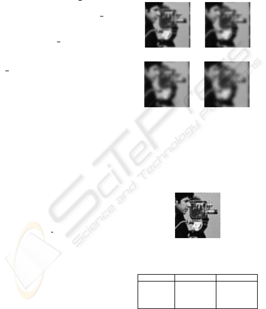
(BSNR) was equal to 40dB and 20dB. Observations
for the 40dB BSNR case are shown in Figure 1.
In order to compare different restorations we
have used Improved Signal to Noise Ratio (ISNR)
as our comparison metric. ISNR is defined as
10log
10
kg
i
− fk
2
/kf
k
− fk
2
.
(a) Channel 1. (b) Channel 2.
(c) Channel 3. (d) Channel 4.
Figure 1: Multi-channel observations (BSNR=40dB).
In order to obtain an upper bound for our blind
multi-channel restoration results, we performed non
blind multi-channel restoration. This restoration re-
sults from setting α
bl,i
= λ
2
= 0 in Equation 15.
The non blind multi-channel based restoration for the
BSNR=40dB observation set is shown in Figure 2 and
the correspondingISNR values in dB are shown in Ta-
ble 1.
Figure 2: Non blind multi-channel restoration (BSNR =
40dB).
Table 1: Non blind restoration ISNR values in dB.
Channel No. BSNR = 40dB BSNR = 20dB
1 9.27 5.08
2 9.17 5.02
3 9.35 5.11
4 9.55 5.32
In order to better understand and to quantify the
information provided by each prior and observation
model we normalized the parameters so that p
1
+p
2
+
VISAPP 2008 - International Conference on Computer Vision Theory and Applications
568

p
3
+ p
4
= 1, where p
1
= α
im
, p
2
= λ
2
ε
bl
, p
3
=
∑
i
α
bl,i
and p
4
=
∑
i
λ
1
β
i
.
We proceeded by setting p
2
equal to zero and by
adjusting p
1
and p
3
to maximize the ISNR of the
restoration. Once p
1
and p
3
were determined, the val-
ues of p
2
and p
4
were varied to determine the signif-
icance of the observation models used in the restora-
tion process.
Tables 2 and 3 show that the ISNR of the restora-
tion obtained by combining the noise and subspace
observation models is greater than the one obtained
by using only the noise observation model. For
the BSNR=40dB set, the improvement on average is
0.66dB and 1.17dB depending on whether we use non
degenerate or degenerate distributions to approximate
the image posterior distribution. This table also shows
that the approximation of the global posterior distri-
bution by a combination of degenerate distribution for
the blur and non degenerate distribution for the image
outperforms the model where both are degenerate.
It is important to understand what is the value that
multiple observations of the same scene bring to the
blind restoration problem. In order to answer this
question we performed blind single channel restora-
tion on the least blurred channel. Tables 4 and 5 show
the corresponding blind single-channel restoration re-
sults. It can be observed that our blind multi-channel
based restoration with optimal random distribution
q(f) outperforms blind-single channel restoration as
well. However, this is not the case for the blind multi-
channel restoration based on the degenerate random
distribution q(f).
It can also be observed that our best blind-multi
channel based restoration for the BSNR=40dB set is
approximately 2.4dB below its upper bound from Ta-
ble 1. The blind multi-channel based restoration with
optimal random distribution q(f) for the BSNR=40dB
observation set is shown in Figure 3.
Figure 3: Blind multi-channel restoration (BSNR = 40dB)
with optimal random distribution q(f).
Table 2: Blind multi channel restoration for the
BSNR=40dB with optimal random distribution q(f).
(p
1
,p
2
,p
3
,p
4
) ISNR [dB]
(1e-4,0,0.12,0.8799) Ch. 1: 6.22
Ch. 2: 6.12
Ch. 3: 6.30
Ch. 4: 6.51
(1e-4,0.5,0.12,0.3799) Ch. 1: 6.88
Ch. 2: 6.78
Ch. 3: 6.96
Ch. 4: 7.16
Table 3: Blind multi channel restoration for the
BSNR=40dB with degenerate random distribution q(f).
(p
1
,p
2
,p
3
,p
4
) ISNR [dB]
(1e-4,0,0.12,0.8799) Ch. 1: 3.18
Ch. 2: 3.08
Ch. 3: 3.26
Ch. 4: 3.46
(1e-4,0.1,0.12,0.7799) Ch. 1: 4.35
Ch. 2: 4.25
Ch. 3: 4.43
Ch. 4: 4.63
Table 4: Blind single channel restoration for the
BSNR=40dB with optimal random distribution q(f).
(p
1
,p
2
,p
3
,p
4
) ISNR [dB]
(1e-4,0,0.12,0.8799) Ch. 1: 5.98
Table 5: Blind single channel restoration for the
BSNR=40dB with degenerate random distribution q(f).
(p
1
,p
2
,p
3
,p
4
) ISNR [dB]
(1e-4,0,0.12,0.8799) Ch. 1: 4.51
5 CONCLUSIONS
In this paper we examined the use of the logarithmic
opinion pooling to statistically combine two observa-
tion models that are regularly used in the multichan-
nel image restoration algorithms. In order to pro-
vide an estimate of the posterior distributions of the
real underlying image and the unknown blurs vari-
ational techniques were used. Variational approxi-
mations lead to two different iterative blind multi-
channel based restoration algorithms. Both of these
algorithms are incorporating some prior assumptions
(e.g. SAR models on unknown image and blurs)
about the unknowns into the restoration process. Ad-
ditionally, both algorithms are incorporating two ob-
servations models into the restoration process, which
USING LOGARITHMIC OPINION POOLING TECHNIQUES IN BAYESIAN BLIND MULTI-CHANNEL
RESTORATION
569

allows us to further constraint unknown blurs in par-
ticular. As can be seen from the experimental section
both multi-channel based restoration algorithms per-
formed better when logarithmic opinion pooling tech-
nique was used to statistically combine observation
models into the restoration process.
ACKNOWLEDGEMENTS
This work has been supported by the Comisi´on
Nacional de Ciencia y Tecnolog´ıa under contract
TIC2007-65533.
REFERENCES
Bishop, T., Babacan, D., Amizic, B., Katsaggelos, A. K.,
Chan, T., and Molina, R. (2007). Blind image de-
convolution: problem formulation and existing ap-
proaches. In Campisi, P. and Egiazarian, K., editors,
Blind image deconvolution: Theory and Applications,
chapter 1, pages 1–42. CRC.
Galatsanos, N. P., Mesarovic, V. Z., Molina, R., Katsagge-
los, A. K., and Mateos, J. (2002). Hyperparameter es-
timation in image restoration problems with partially-
known blurs. Optical Eng., 41(8):1845–1854.
Gastaud, M., Ladjal, S., and Matre, H. (2007). Blind fil-
ter identification and image superresolution using sub-
space methods. In European Signal Processing Con-
ference. Poznan (Poland).
Genest, C. and Zidek, J. V. (1986). Combining probability
distributions: A critique and an annotated bibliogra-
phy. Statistical Science, 1:114148.
Katsaggelos, A., Molina, R., and Mateos, J. (2007). Super
resolution of images and video. Synthesis Lectures
on Image, Video, and Multimedia Processing. Morgan
and Claypool.
Kullback, S. (1959). Information Theory and Statistics.
New York, Dover Publications.
Kullback, S. and Leibler, R. A. (1951). On information and
sufficiency. Annals of Mathematical Statistics, 22:79–
86.
Mateos, J., Katsaggelos, A., and Molina, R. (2000). A
Bayesian approach to estimate and transmit regu-
larization parameters for reducing blocking artifacts.
9(7):1200–1215.
Molina, R., Katsaggelos, A. K., and Mateos, J. (1999).
Bayesian and regularization methods for hyperparam-
eter estimation in image restoration. 8(2):231–246.
Molina, R., Mateos, J., and Katsaggelos, A. (2006). Blind
deconvolution using a variational approach to parame-
ter, image, and blur estimation. IEEE Trans. on Image
Processing, 15(12):3715–3727.
Ripley, B. D. (1981). Spatial Statistics, pages 88–90. John
Wiley.
Sroubek, F., Crist´obal, G., and Flusser, J. (2007). A unified
approach to superresolution and multichannel blind
deconvolution. IEEE Transactions on Image Process-
ing, 9:2322–2332.
VISAPP 2008 - International Conference on Computer Vision Theory and Applications
570
