
LIMITED ANGLE IMAGE RECONSTRUCTION USING FOUR
HIGH RESOLUTION PROJECTION AXES AT CO-PRIME
RATIO VIEW ANGLES
Anastasios L. Kesidis
Computational Intelligence Laboratory, Institute of Informatics and Telecomunications,
National Center for Scientific Research “Demokritos”, GR-153 10 Agia Paraskevi, Athens, Greece
Keywords: Image reconstruction, limited angle tomography, coprime view angles, inverse problems.
Abstract: This paper proposes a sequential image reconstruction algorithm for the exact reconstruction of an image
from a limited number of projection angles. Specifically, four projection axes oriented at coprime ratio view
angles are used. The set of proper values for the view angles as well as the overall number of samples on the
projection axis are explicitly defined and are related only to the dimensions of the image. The slopes of the
four projection axes are calculated according to the chosen view angle and are symmetrically oriented with
respect to the horizontal and the vertical axis. The reconstruction is a non-iterative, one pass process based
on a decomposition sequence which defines the order in which the image pixels are restored. Several
simulation results are provided that demonstrate the feasibility of the proposed method.
1 INTRODUCTION
Computerized tomography (CT) is an important and
effective tool for a large number of imaging
applications allowing the observation of the internal
structure of objects. The majority of applications
refer to the medical sciences including x-ray
tomography, magnetic resonance imaging, electron
microscopy tomography, and diagnostic radiology.
(CT) is also extensively used in the industry for non-
destructive evaluation allowing the determination of
defects and abnormalities in industrial objects. In
general, the object is reconstructed from the
projection data acquired by projecting it into several
fairly equidistant view angles. However, there are
several cases in which projection data can be
acquired only in a limited range of projection view
angles. The limited angle tomography problem
concerns a wide range of applications in surgical
imaging, dental radiology and positron emission
mammography as well as in electron microscopy
and in astronomy. It is well known that applying the
conventional filtered backprojection reconstruction
method and assuming zero values for the missing
view angles produces approximations of the original
image containing significant artefacts (Natterer,
2001). Several approaches have been proposed that
address this problem including sinogram techniques,
Bayesian methods, projections onto convex sets,
maximum entropy techniques and many others.
Recently, Rantala et al (Rantala, 2006) addressed the
reconstruction from limited angle data by using a
wavelet expansion approximation and Besov space a
priori information in order to compute a maximum a
posteriori estimation for the original image. A pre-
thresholding method is also proposed in which
thresholding is applied to the wavelet coefficients
prior to the computation of the reconstruction.
Delaney and Bresler (Delaney, 1998) formulate the
reconstruction problem as a regularized weighted
least-squares optimization problem, and propose a
family of regularization functionals that are meant to
apply a constraint of piecewise smoothness on the
image. Clackdoyle et al (Clackdoyle, 2004) focus on
2-D reconstruction processes where data from entire
projection directions are unmeasured or unavailable
and state that region-of-interest reconstruction from
these truncated projections is possible under certain
conditions. Both direct and statistically based
(iterative) reconstruction algorithm can be used for
the image reconstruction. Schule et al (Schule, 2005)
describe how multi-valued objects can be
reconstructed by combining binary decisions. They
use convex-concave regularization to improve the
reconstruction quality as well as the EM-algorithm
50
L. Kesidis A. (2008).
LIMITED ANGLE IMAGE RECONSTRUCTION USING FOUR HIGH RESOLUTION PROJECTION AXES AT CO-PRIME RATIO VIEW ANGLES.
In Proceedings of the Third International Conference on Computer Vision Theory and Applications, pages 50-57
DOI: 10.5220/0001086300500057
Copyright
c
SciTePress

to motivate the adaption of the absorption
coefficients as hidden data estimation.
In this paper we propose a method for exact
image reconstruction when a limited number of
projections axes (i.e. four) is available that consists
of projection samples with higher resolution than the
pixels of the reconstructed image. Reconstruction
under such conditions may occur in cases where it is
very hard to obtain projections; however, it is
possible in these projections to use high resolution
detectors, or in cases that is not necessary to
reconstruct high resolution images. Examples of
such cases are in surgical imaging, in imaging
nuclear waste cites or in non destructive testing.
More specifically, we propose a method that allows
the exact reconstruction of an image assuming four
projection axes oriented at coprime ratio view
angles. The original grayscale image is projected
into the four projection axes and the collected
projection data are stored in an accumulator array.
The set of proper values for the view angle as well
as the overall number of samples on the projection
axis are related only to the dimensions of the image.
The slopes of the four projection axes are calculated
according to the chosen view angle and are
symmetrically oriented with respect to the horizontal
and vertical axes. The reconstruction is a non-
iterative, one pass process that uses a decomposition
sequence which defines the order in which the image
pixels are restored. The decomposition sequence is
determined so that, a unique correspondence
between a pixel in the exterior of the image and a
projection ray that intersects only this pixel, is
preserved during the reconstruction process.
Initially, the determination of the view angle and the
decomposition sequence is based on the pixels in the
1
st
octant of the image. However, during the
reconstruction process, the symmetrical geometric
properties of the pixels in the other octants are used
in order to restore all the image’s pixels.
The rest of this paper is organized as follows:
Section 2 presents an initial approach to determine a
proper view angle that allows the exact
reconstruction of the image. Besides the view angle,
certain projection parameters are also defined that
determine the geometry of the reconstruction
utilization. In section 3 we extend the methodology
in order to determine a set of several other coprime
ratio view angles that can also be used in the
proposed reconstruction scheme. We provide
generalized versions of the projection parameters
that are related only to the image dimensions and the
slope of the projection axis. Time and memory
complexity issues are also considered and the
applicability of the proposed method using various
projection view angles is also demonstrated. Finally,
section 4 draws the conclusion.
2 AN INITIAL APPROACH FOR
EXACT IMAGE
RECONSTRUCTION
2.1 Accumulator Array
Without loss of generality let us suppose an input
image I of size N×N pixels where N is assumed to be
an even positive integer. A pixel in the input image
at position (i,j) has grayscale (intensity) value I(i,j),
with i, j = −N/2…N/2−1, and is assumed to be a
square area of unit size with constant intensity value.
The projection data obtained by projecting the image
into K
θ
projection axes is stored in an accumulator
array C. Each projection axis consists of a finite
number of projection rays s
l
where l=1,2,…,K
l
.
Clearly, each sample in array C(θ,s) corresponds to a
projection ray identified by the combination of the
slope θ
k
with the displacement value s
l
. If I
θ,s
denotes
the set of image pixels that a projection ray r
θ,s
intersects, then for each pixel (i,j)∈I
θ,s
we define the
weighting factor w
θ,s
(i,j) to be the area of the portion
of r
θ,s
inside pixel (i,j). Thus, each sample of C is
calculated as
C(θ,s)=
∑
∈
s
Iji
s
jiwjiI
,
),(
,
),(),(
θ
θ
(1)
2.2 Projection Parameters
Determination
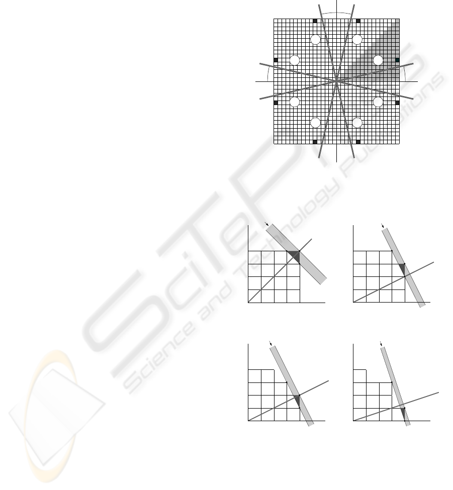
The image is divided into 8 octants as shown in Fig.
1 where the gray shaded pixels denote the 1
st
octant.
A pixel (i,j) in the 1
st
octant has coordinates
0≤i≤N/2−1, 0≤j≤i. The black pixels in Fig. 1 denote
pixels in all octants that have symmetrical geometric
properties. There are also K
θ
=4 projection axes
shown at slopes
θ
k
=( uuuu −+−
π
π
π
,
2
,
2
, ) for k=1…K
θ
(2)
where u is the projection view angle. The following
discussion refers to pixels in the 1
st
octant and will
be later generalized for the pixels in all octants based
on the symmetrical positioning of the pixels
relatively to the image’s center.
LIMITED ANGLE IMAGE RECONSTRUCTION USING FOUR HIGH RESOLUTION PROJECTION AXES AT
CO-PRIME RATIO VIEW ANGLES
51

Let us consider the four instances shown in Fig.
2 as the first steps of a decomposition sequence
regarding the pixels in the 1
st
octant. By convention,
the diagonal pixels are attributed to the odd octants.
The decomposition sequence refers to pixels in the
last column of the 1
st
octant, namely pixels (i,i−n),
where i=N/2−1 and n=0…i denotes an positive offset
from the diagonal. Our intention is to identify the
width of the projection ray as well as its
displacement on the projection axis that provide the
largest possible intersection area without intersecting
any other pixel of the current or the adjacent octant
(octants 1 and 2 in this case). Lines r
1
and r
2
are
perpendicular to the projection axis and define the
boundaries of the projection ray. For each n, the
intersection between projection ray r
θ,s
and pixel
(N/2−1, N/2−1−n) is considered. For all forthcoming
values of n, the pixel just examined and its
counterpart in the 2
nd
octant are ignored. Hence, in
Fig. 2b pixel (i,i) is ignored, and pixel (i,i−1) is
considered. Clearly, any line r
2
further away from
the origin does not affect the intersection area. On
the other hand, if line r
1
is shifted in parallel towards
the origin then pixels (i−1,i) and (i,i−2) are also
intersected by projection ray r
θ,s
which is
undesirable. Again, in the following steps pixel
(i,i−1) as well as its counterpart in 2
nd
octant, pixel
(i−1,i), are ignored.
The process is repeated in Figs. 2c and 2d for
pixels (i,i−2) and (i,i−3), respectively. As shown in
Fig. 2d line r
1
is determined by points p
1
and p
3
and
is the closest to the origin line for which the
projection ray intersects only pixel (i,i−n). Line r
2
is
a line parallel to r
1
that intersects the upper right
vertex of pixel (i,i−n), namely point p
2
. It can be
noticed that for n>1 point p
3
corresponds to the
upper right vertex of pixel (i−1,i−1) while points p
1
and p
2
are related to n. Setting i=N/2−1 and n=i, and
based on the geometry of the utilization as shown in
Fig. 2d allows the determination of the projection
parameters
u=arctan(2/(N-2)), d=2/
84
2
+− NN ,
w=1/(N-2), K
p
=
Ν
/2 and K
l
= 2/
2
N
(3)
where u is the view angle of the projection axis, d
denotes the width of each projection ray, w is the
area between any pixel and the furthest from the
origin projection ray that intersects it, while K
p
and
K
l
denote the number of rays that intersect a pixel
and the overall number of samples on the projection
axis, respectively. These parameters are related only
to the image dimension N. The weighting factor
w
θ,s
(i,j) in (1) equals
{
}
⎩
⎨
⎧
==
=
otherwise2
orif
),(
,
w
ssssw
jiw
fc
s
θ
(4)
where s
c
and s
f
denote the nearest and furthest from
the origin projection ray that intersect pixel (i,j),
respectively.
2.3 Image Reconstruction
Let us suppose that the original image is projected
onto the four projection axes each one consisting of
K
l
samples. The overall projection data, i.e. K
θ
K
l
samples, are stored in accumulator array C. In the
following we present how the original image can be
exactly reconstructed from the samples in array C.
Let
I
R
denote the reconstructed image. In section 2.2
we stated that the main criterion for the
determination of the projection parameters is that the
furthest from the origin projection ray that intersects
a pixel does not intersect the upper right area w of
any other pixel in the same octant. Thus for each
pixel (i,j) there is a specific sample at slope θ
k
and
displacement value s
l
that corresponds to this
projection ray. This sample is used in order to
determine the corresponding pixel’s grayscale value
I
R
(i,j). Having obtained its value, the pixel’s
contribution is removed from the accumulator array
i.e., all the samples of C affected by this pixel
decrease their value by an amount proportional to
the weighting factor w
θ,s
(i,j).
The order in which the pixels are examined is
given by a decomposition sequence T
1
{t} initially
defined for the pixels in the 1
st
octant. The sequence
T
1
{t} contains the pixels of the 1
st
octant sorted
column wise from the periphery to the inner of the
image, i.e. pixels (N/2−1, N/2−1), (N/2−1, N/2−2),
…, (N/2−1, 0), (N/2−2, N/2−2), (N/2−2, N/2−3),…
etc, down to (0,0). For each pixel of the
decomposition sequence its symmetric counterparts
in the other octants are also examined before the
decomposition continues with the next sequence
element. The reconstruction process starts with the
first member of T
1
{t}, pixel (i,j)=(N/2−1, N/2−1).
Let
),( jis
f
denote the furthest from the origin
projection ray of projection axis θ
1
that intersects
pixel (i,j). For
θ
ˆ
=θ
1
and s
ˆ
=
),( jis
f
projection ray
s
r
ˆ
,
ˆ
θ
intersects only pixel (i,j). The accumulator array
sample C(
θ
ˆ
, s
ˆ
), that holds the value of projection
VISAPP 2008 - International Conference on Computer Vision Theory and Applications
52

ray
s
r
ˆ
,
ˆ
θ
, equals the weighted portion ),(
ˆ
,
ˆ
jiw
s
θ
of
pixel’s (i,j) grayscale value. Hence, pixel I
R
(i,j) in
the reconstructed image can be calculated as
I
R
(i,j)=
),(
)
ˆ
,
ˆ
(
ˆ
,
ˆ
jiw
sC
s
θ
θ
for
θ
ˆ
=θ
1
and
s
ˆ
=
),( jis
f
(5)
After the determination of I
R
(i,j) the contribution of
pixel (i,j) is removed from the other samples of C.
Specifically, if P
θ
(i,j) denotes the set of projection
rays r
θ,s
that intersect pixel (i,j) at any angle θ
k
then
the accumulator array is updated as follows
C(θ,s) ← C(θ,s)
−
I
R
(i,j)w
θ
,
s
(i,j)
(6)
for {(θ,s) : r
θ,s
∈ P
θ
(i,j)}.
So far, we considered pixels in the 1
st
octant.
Applying proper re-indexing allows the
manipulation of pixels in all other octants. Thus,
before continuing with the next member of T
1
{t} the
above process is applied to pixels in the other
octants that are symmetrical to pixel (i,j). There are
four or eight of them depending on whether pixel
(i,j) lies on the diagonal axis or not. Thus, if M
T
(i,j)
denotes the set of pixels that are symmetrical to
pixel (i,j) then
{}
{
}
⎪
⎪
⎩
⎪
⎪
⎨
⎧
≠−−−−−−−−
−−−−−−−−
=−−−−−−−−
=
jiji,ij,i,j
j,ijiijijji
jiiiiiiiii
jiM
T
if)1( ),1( ),11(
),11( ),,1( ),,1( ),,( ),,(
if)1,(),1,1(),,1(),,(
),(
(7)
The process continues with the next element of the
decomposition sequence until all the pixels in all
octants are examined. Finally, the accumulator array
becomes empty and the reconstructed image equals
the original one, that is, corresponding pixels in I
and I
R
have identical intensity values.
3 GENERALIZATION FOR
RATIONALLY SLOPED
PROJECTION AXES
In this section we show that the determination of the
decomposition sequence T
1
{t} by sorting the pixels
column-wise from the periphery to the inner of the
image is not unique. In fact, it corresponds to a
special case of a general set of parameter settings
that allow the reconstruction of the image from
several other projection axes that are rationally
sloped.
3.1 Projection Slope Determination
In the following by projection line we mean a line
that defines the border between adjacent projection
ray, e.g. lines r
1
and r
2
in Fig.2. Also, the term
lattice points refers to points on the image plane that
correspond to the upper right vertex of the pixels in
the 1
st
octant. Let p
3
(a)=(N/2−a, N/2−a) be a lattice
point corresponding to the upper right vertex of a
diagonal pixel with offset a relatively to lattice point
(N/2,N/2). Points p
3
(a) and p
1
=(N/2,0) form a
projection line with slope
m
=
)(
)(
,1,3
,1,3
app
app
xx
yy
−
−
=1−
a
N
2
(8)
The view angle u of a projection axis perpendicular
to m is given by
u
=arctan(−
m
1
)=arctan
⎟
⎠
⎞
⎜
⎝
⎛
− aN
a
2
2
(9)
Since the range of view angles in the 1
st
octant is
0
≤u≤π/4 it follows from (9) that valid integer values
for offset a are in the range
a
∈
{1…
⎣
⎦
4/N }
(10)
where symbol
⎣
⎦
x stands for the largest integer less
than or equal to x.
Our intention in the selection of a proper slope m
(which in turn affects the value of the perpendicular
view angle u) is to form a utilization of adjacent
projection rays in such a way that the upper right
area of each pixel in the 1
st
octant is intersected by
only one projection ray. Reconsidering the example
in Fig. 2d it is clear that the slope of the projection
ray is m
=−3 which follows from (8) for N=8 and
a
=1. It can be noticed that for a=1, projection line
l
=r
1
intersects only one lattice point in the 1
st
octant,
that is p
3
(a)=(N/2−1, N/2−1). This is not the case for
all values of a. Our main requirement that only one
projection ray intersects each pixel’s upper right area
can be interpreted as a requirement for the projection
line l connecting points p
3
(a) and p
1
to intersect only
one lattice point. Indeed, if line l intersects more
than one lattice points then the projection ray that
follows l intersects the upper right area of more than
one pixel in this octant. This can be clearly seen in
the examples of Fig. 3b and 3d. Therefore, from all
⎣
⎦
4/N possible values of offset a we concern only
those for which point p
3
(a) is mutual visible from
point p
1
as in the case of Fig. 3a and 3c.
LIMITED ANGLE IMAGE RECONSTRUCTION USING FOUR HIGH RESOLUTION PROJECTION AXES AT
CO-PRIME RATIO VIEW ANGLES
53

Typically, two lattice points (x
a
,y
a
) and (x
b
,y
b
) are
mutually visible if the line segment joining them
contains no further lattice points (Boca, 2000).
Moreover, they satisfy the relation gcd(x
b
−x
a
,
y
b
−y
a
)=1, where gcd(a,b) denotes the greatest
common divisor of a and b. In our case this
corresponds to
gcd(p
1,x
−p
3,x
, p
1,y
−p
3,y
)
=
gcd(a,a
−
N/2)=
=gcd(a,N/2)=1
(11)
This is an important relation in our method since it
states that p
3
(a) and p
1
are mutually visible if offset
a is coprime to N/2. Let F
N
denote the set of all
values of a for which the above relation holds, that is
F
N
=
⎣⎦
{}
1)2/,gcd(and4/: =≤ NaNaa
(12)
The cardinality K
a
of F
N
is given by the Euler
function φ(n). Function φ(n), also known as totient
function (Finch, 2003), is defined as the number of
positive integers less than or equal to n that are
relatively prime to n, that is
φ(n)
= #{a∈N: a≤n and gcd(a,n)=1}
(13)
where 1 is counted as being relatively prime to all
numbers. For a prime p it is φ(p)
=p−1 since all
numbers less than p are relatively prime to p. Since
a
≤
⎣⎦
4/N the overall number of proper offset values
is
K
a
=
()
2
2/N
ϕ
(14)
Indeed, for N
=16, it is F
N
={1,3}, K
a
=2 and (8) gives
m
=−7/1 and m=−5/3 as shown in Fig. 3a and 3c.
Summarizing, if the image is projected on a
projection axis at angle u given by (9) for a
∈F
N
then
each projection ray does not intersect the upper right
area of more than one pixel in the 1
st
octant.
3.2 Determination of the other
Projection Parameters
The width d of the projection ray is given by the
width of the broadest projection ray that does not
contain any lattice points of the 1
st
octant in its
interior. Indeed, if one or more lattice points are
contained in the projection ray then the upper right
area of more that one pixels are intersected by this
specific projection ray, which contradicts our main
hypothesis. It can be shown that, if the projection
lines have a direction tanθ
=m=a/b, with gcd(a,b)=1
then there are projection ray paths of width d>0
containing no lattice points (Olds, 2001). The width
of the broadest such ray is
d
=
22
ba
bqap
+
+
=
22
),gcd(
ba
ba
+
=
22
1
ba +
(15)
We have already defined point p
3
(a) as a lattice
point in the diagonal with offset a from point (N/2,
N/2). Hence b
= N/2−a and the above equation results
to
d
=
22
84
2
aaNN +−
(16)
This equation provides the width of each projection
ray (and consequently the width of the samples on
the projection axis) as a function of offset a.
According to Fig. 4 the area of the triangle that
forms the intersection between a projection ray and
the upper right area of a pixel equals
w
=
2
))(( KLML
=
uu
d
cossin2
2
=
u
d
2sin
2
(17)
Using equations (9) and (16) this can be written as a
function if a as
w
=
⎟
⎠
⎞
⎜
⎝
⎛
−
+− )
2
2
arctan(2sin)84(
4
22
aN
a
aaNN
=
=
aaN )2(
1
−
(18)
The intersection area w
θ,s
(i,j) between any pixel (i,j)
and a projection ray perpendicular to angle θ
k
and
displacement s can be calculated as a multiple of w.
Indeed, as shown in Fig. 4, any intersection area can
be constructed as a sum of one or more right
triangles of area w. For a projection axis at angle
tan(θ)
=a/b, where a, b are coprime numbers with
a<b and b≠0, the displacement k inside the pixel’s
area is
k
=
⎩
⎨
⎧
≤≤−
otherwise0
if
fcc
sssss
(19)
with s
c
=aj+bi and s
f
=s
c
+K
p
−1. The number of
triangles inside the projection area is given by
m(k)
=
⎪
⎩
⎪
⎨
⎧
−≤≤−−
<≤
<≤+
1if1)(2
if2
0if12
pp
KkbkK
bkaa
akk
(20)
Hence, the intersection area in the k-th displacement
is
w
θ
,
s
(i,j)
=
m(k)w
(21)
VISAPP 2008 - International Conference on Computer Vision Theory and Applications
54

Equation (18) implies also that for given image
dimension N, the area w is maximum for a
=1 and
decreases as a reaches
⎣⎦
4/N . Regarding the
parameters K
p
and K
l
it follows from Fig. 4 that
K
p
=
d
CF)(
=
d
uu )sin()cos( +
=
2
N
(22)
and
K
l
=
Ν
K
p
=
2
2
N
(23)
These relations are in accordance with (3) and show
that the number of projection ray intersecting each
pixel as well as the overall number of samples in the
projection axis do not dependent on offset a.
3.3 Image Reconstruction
The reconstruction methodology described in section
2.3 can be applied for any value of a∈F
N
. Indeed,
equations (9), (16) and (18) provide the view angle
u, the width of the projection ray d and the
intersection area w as a relation of image dimension
N and offset a. Thus, if the original image is
projected onto four projection axes whose
parameters are defined by these relations then the
original image pixels can be recovered from
accumulator array C. The process described in
section 2.3 can be considered as a special utilization
using parameter settings calculated for a=1.
However there is a significant difference concerning
the decomposition sequence. In section 2.3 sequence
T
1
{t} is defined by the pixels of the 1
st
octant sorted
column-wise from the periphery to the inner of the
image. In its general form, the decomposition
sequence T
a
{t} holds the pixels of the 1
st
octant
sorted decreasingly according to their s
f
value, that is
the furthest from the origin projection ray that
intersects each pixel. Fig. 5 depicts two
decomposition sequences for N=16. On the left
example, it is a=1 while on the right example, the
offset is a=3 resulting to a different re-ordering of
the pixels in the decomposition sequence.
Fig. 6 depicts the reconstruction of the well
known phantom image (Shepp, 1974) of size
N×N=256×256 pixels using three different view
angles. The image is projected into four projection
axes given by (2) which are symmetrically oriented
with respect to the horizontal and vertical axis, as
shown in Fig. 1. In all the cases the pixels in the
periphery of the image are reconstructed first
followed by the pixels in the center of the image. For
each pixel in the decomposition sequence its
symmetrical pixels in the other octants are also
reconstructed leading to a symmetrical outer-to-
inner reconstruction of the image. However, the
order in which the pixels are considered depends on
the view angle u which, in turn, is directly related to
the applied offset value. In the left column of Fig. 6
the image is reconstructed using an offset value a=1
which corresponds to a view angle u=0.45
o
. It can be
clearly seen that pixels are reconstructed column-
wise or row-wise, depending on the octant in which
the process is applied. In the middle and the right
column the offset values are a=23 and a=63,
corresponding to view angles u=12.36
o
and
u=44.10
o
, respectively. The later is the highest value
of a that can be used for the given image dimensions
according to (12). Clearly, there is a different
decomposition sequence for any of the K
a
available
values of a, but all of them lead finally to the exact
reconstruction of the original image. It should be
also noticed, that if N=2p where p a prime number
then according to (14) there is a maximum of
K
a
=
(p
−
1)/2
=
(N−2)/4
(24)
available offset values and consequently (N−2)/4
different view angles u according to which the four
projection axes can be oriented.
3.4 Complexity and Applicability
Let n=N
2
denote the overall number of pixels in the
image. The memory requirements of the proposed
methods is O(n). Indeed, the accumulator array
requires K
θ
K
l
=4(n/2) =2n memory units and there
are n/8 entries in decomposition sequence
}{tT
a
.
Considering time complexity, the most consuming
processes are the decomposition sequence
determination and the reconstruction process.
Although sorting the pixels during the determination
of
}{tT
a
is O(n
2
) in the worst case, the average time
is O(nlogn) (Havil, 2003). The complexity for the
reconstruction process is related to the
decomposition of the accumulator array C which is
O(n
n
). It should be noticed that }{tT
a
is not
related to the image’s contents. Therefore, it is not
necessary to determine the decomposition sequence
each time an N×N image is considered. Instead, it
can be determined once for a given set of parameter
settings N and a
k
and then retrieved from a lookup
table anytime an image with the same parameters is
considered.
LIMITED ANGLE IMAGE RECONSTRUCTION USING FOUR HIGH RESOLUTION PROJECTION AXES AT
CO-PRIME RATIO VIEW ANGLES
55
4 CONCLUSIONS
In this paper we presented a sequential
reconstruction method that allows the exact
reconstruction of an image when it is projected into
four projection axes which are symmetrically
oriented with respect to the horizontal and the
vertical axis at coprime ratio view angles. Analytical
relations are provided that determine the parameter
settings, namely the set of proper view angles, the
density of samples in each projection axis and the
intersection area between a pixel and a projection
ray. The chosen view angle affects the
decomposition sequence which determines the order
in which the pixels are restored. The image is
reconstructed by a one pass decomposition process
where the external pixels are restored first followed
by the pixels in the image’s center. It should be
noticed that we addressed the proposed method as a
quantitative reconstruction process problem and did
not considered optimization of noise propagation.
Future work includes a detailed analysis of the
algorithm’s behavior when noisy data are present as
well as the formulation of the proposed method in an
increasingly detailed hierarchical reconstruction
approach.
REFERENCES
Boca, F. P., Cobeli, C, Zaharescu, A. , 2000. Distribution
of Lattice Points Visible from the Origin. In Comm.
Math. Phys., vol 213, pp. 433-470.
Clackdoyle, R., Noo, F., Guo, J., Roberts, J. A. , 2004.
Quantitative reconstruction from truncated projections
in classical tomography. In IEEE Trans. Nucl. Sci.,
vol. 55(2), pp. 2570-2578.
Delaney, A. H., Bresler, Y., 1998. Globally convergent
edge-preserving regularized reconstruction: an
application to limited-angle tomography. In IEEE
Trans. Image Process., vol. 7, pp. 204–221.
Finch, S. R., 2003. Euler Totient Constants. In
Mathematical Constants. Cambridge University Press,
pp. 115-119.
Havil, J., 2003. Quicksort Gamma: Exploring Euler's
Constant, Princeton University Press, pp. 128-130.
Natterer, F. , 2001 The Mathematics of Computerized
Tomography. Philadelphia, SIAM.
Olds, C. D., Lax, A., Davidoff, G. P., 2001. The Geometry
of Numbers, The Mathematical Association of
America.
Rantala, M., Vanska, S., Jarvenpaa, S., Kalke, M., Lassas,
M., Moberg, J. Siltanen, S., 2006. Wavelet-based
reconstruction for limited-angle X-ray tomography. In
IEEE Trans. Med. Imag., vol 25 (2), pp. 210-217.
Schule, T., Weber, S., Schnorr, C., 2005. Adaptive
Reconstruction of Discrete-Valued Objects from few
Projections. In Electronic Notes in Discrete
Mathematics, vol. 20, pp. 365-384.
Shepp, L. A., Logan, B. F., 1974. The Fourier
reconstruction of a head section. In IEEE Trans. Nucl.
Sci., vol. 21, pp. 21-43.
u
uu
u
1
23
4
5
6 7
8
Figure 1: The image is divided into eight octants. The gray
shaded pixels denote the 1st octant. The black pixels
denote pixels with symmetrical geometric properties.
0
0
N/2-1
N/2-1
r
θ
,s
r
1
r
2
p
3
p
1
p
2
0
0
N/2-1
N/2-1
r
θ
,s
r
1
r
2
p
3
p
1
p
2
(a) (b)
0
0
N/2-1
N/2-1
r
θ
,s
r
1
r
2
p
3
p
1
p
2
0
0
N/2-1
N/2-1
r
θ
,s
r
1
r
2
p
3
p
1
p
2
(c) (d)
Figure 2: Intersection of a projection ray and the pixel (i,
i−n) in the 1
st
octant of an N×N=8×8 pixels image. Four
cases are shown where i=N/2−1 and n=0, 1, 2 and 3,
respectively. In each case the light shaded strip depicts the
projection ray and the dark shaded area denotes the
intersection between the pixel and the projection ray.
VISAPP 2008 - International Conference on Computer Vision Theory and Applications
56
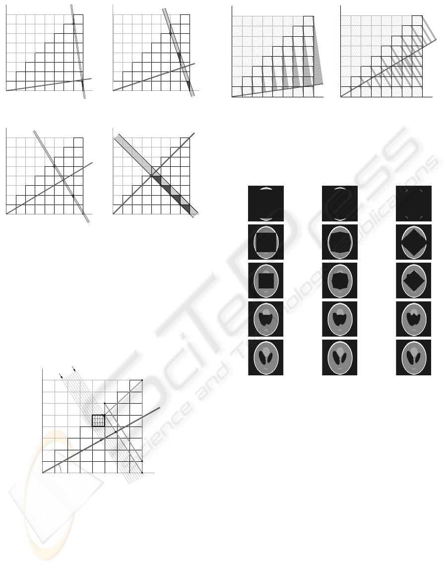
p
3
p
1
p
2
l
a
=1
p
3
p
1
l
a
=2
(a) (b)
p
3
p
1
p
2
l
a
=3
p
3
p
1
l
a
=4
(c) (d)
Figure 3: The number of pixels whose upper right area is
intersected by a projection line equals the number of
lattice points of the 1
st
octant joining the line segment l
between p
3
(a) and p
1
(denoted by a circle). There is a
unique such pixel if offset a is coprime to N/2 (subfigures
(a) and (c)), and more than one, otherwise (subfigures (b)
and (d)). In any case the dark shaded area denotes the
intersection between the upper right area of a pixel and the
projection ray.
i
j
u
s
c
s
f
{
K
p
C
F
LM
K
D
G
H
E
Figure 4: Each pixel is intersected by K
p
projection rays.
The dark shaded area denotes the intersection between
pixel (i,j) and the projection ray s
f
that is the furthest from
the origin ray that intersects the pixel.
1
2
3
4
5
6
7
8
9
10
11
12
13
14
15
16
17
18
19
20
21
22
23
24
25
26
27
28
29
30
31
32
33
34
3536
N
=16,
a
=1
1
2
3
4
5
6
7
8
9
10
11
12
13
14
15
16
17
18
19
20
21
22
23
24
25
26
27
28
29
30
31
32
33
34
35
36
N
=16,
a
=3
(a) (b)
Figure 5: Decomposition sequence T
a
{t} of an
N×N=16×16 sized image for (a) a=1 and (b) a=3. In each
case the pixels are sorted according to the furthest from
the origin projection ray that intersects them.
(a)
(b)
(c)
Figure 6: Reconstruction of a 256×256 phantom image
using three different projection angles. The offset values
are (a) a=1, (b) a=23 and (c) a=63. In each case, the
symmetrical orientation of the four projection axes around
the horizontal and the vertical axis result to an outer-to-
inner reconstruction of the image.
LIMITED ANGLE IMAGE RECONSTRUCTION USING FOUR HIGH RESOLUTION PROJECTION AXES AT
CO-PRIME RATIO VIEW ANGLES
57
