
USE OF SPATIAL ADAPTATION FOR IMAGE RENDERING
BASED ON AN EXTENSION OF THE CIECAM02
Olivier Tulet, Mohamed-Chaker Larabi and Christine Maloigne Fernandez
SIC Laboratory, University of Poitiers
Bat. SP2MI, Téléport 2, BP 30179, 86962 – FUTUROSCOPE Chasseneuil Cedex, France
Keywords: Rendering model, image quality, subjective assessment, spatial frequencies, s-CIECAM.
Abstract: With the development and the multiplicity of imaging devices, the color quality and portability have
become a very challenging problem. Moreover, a color is perceived with regards to its environment. In
order to take into account the variation of perceptual vision in function of environment, the CIE
(Commission Internationale de l'éclairage) has standardized a tool named color appearance model
(CIECAM97*, CIECAM02). These models are able to take into account many phenomena related to human
vision of color and can predict the color of a stimulus, function of its observations conditions. However,
these models do not deal with the influence of spatial frequencies which can have a big impact on our
perception. In this paper, an extended version of the CIECAM02 was presented. This new version integrates
a spatial model correcting the color in relation to its spatial frequency and its environment. Moreover, a
study on the influence of the background’s chromaticity has been also performed. The obtained results are
sound and demonstrate the efficiency of the proposed extension.
1 INTRODUCTION
In order to answer the constant evolution in the
domain of color appearance and image rendering,
many rendering models have appeared. These
models become more and more complex and give a
good simulation of the human vision. They are often
based on color appearance models (CAM) that allow
the decomposition of a color into perceptual features
based on the environment.
Several CAMs exist and are dedicated to
different applications. They take into account several
visual phenomena like chromatic adaptation,
simultaneous contrast, crispening, spreading…
These models answer the request of industries
which asked for standardized tools. It is for this
reason, that the CIE has normalized in 1997 the
CIECAM97 which has been thereafter improved in
order to lead to the CIECAM02 (Fairchild 1997).
Thus, these models allow correcting many
phenomena that modify the appearance of a color
stimulus (Moroney, Fairchild, Hunt, C.J Li, Luo, and
Newman 2002, Luo and Hunt 1997). However they
do not take into account the spatial aspect that can
be contained in a stimulus (Johnson 2005, Wandell
1995).
As a first contribution to the CIECAM02, we
have integrated a model that deals with both spatial
frequencies and background luminance. The
obtained results were very encouraging since the
appearance of the stimuli was adapted to the
contained spatial frequency. However, this model
addressed only a single input color and was unable
to correct the content of an image which is more
complex (Larabi and Tulet 2006).
It is to respond to this lack that an image
extension of this model is proposed in this paper.
This extension is carried out by using Fourier
decomposition in different frequency bands. Indeed,
in this space, it is possible to have a direct access to
the orientation and the energy for all the frequencies.
A study of the neighborhood and the orientation of a
pixel allow extracting the background luminance
that will be used to correct the pixel.
The main difference between the proposed model
and the other rendering models like the iCAM
developed by Fairchild et al. (Fairchild and Johnson
2004) lies in the fact of taking into account the
spatial repartition of a pixel in addition to its
environment. The others rendering model are just
using a general CSF filter to take into account the
spatial information and are not looking to the
128
Tulet O., Larabi M. and Maloigne Fernandez C. (2008).
USE OF SPATIAL ADAPTATION FOR IMAGE RENDERING BASED ON AN EXTENSION OF THE CIECAM02.
In Proceedings of the Third International Conference on Computer Vision Theory and Applications, pages 128-133
DOI: 10.5220/0001086101280133
Copyright
c
SciTePress
environment of each pixel.
The remainder of this paper is organized as follows:
Section 2 describes the model already developed and
the experiments which allowed its construction. A
recent study of the influence of background
chromaticity, on spatial frequencies, is exposed.
Section 3 is dedicated to the extension of this s-
CIECAM model to images. In this last section some
results are described and different tests to validate
our method are realized. We finish by some
conclusions and we introduce some future works.
2 S-CIECAM FRAMEWORK
An extension of the CIECAM02 has been developed
in order to allow this color appearance model takes
into account the influence that can have the spatial
frequencies on our vision.
For that a study based on psychophysical
experiments has been realized in a dedicated room.
This room respects standardized conditions
(lightness, display calibration…).
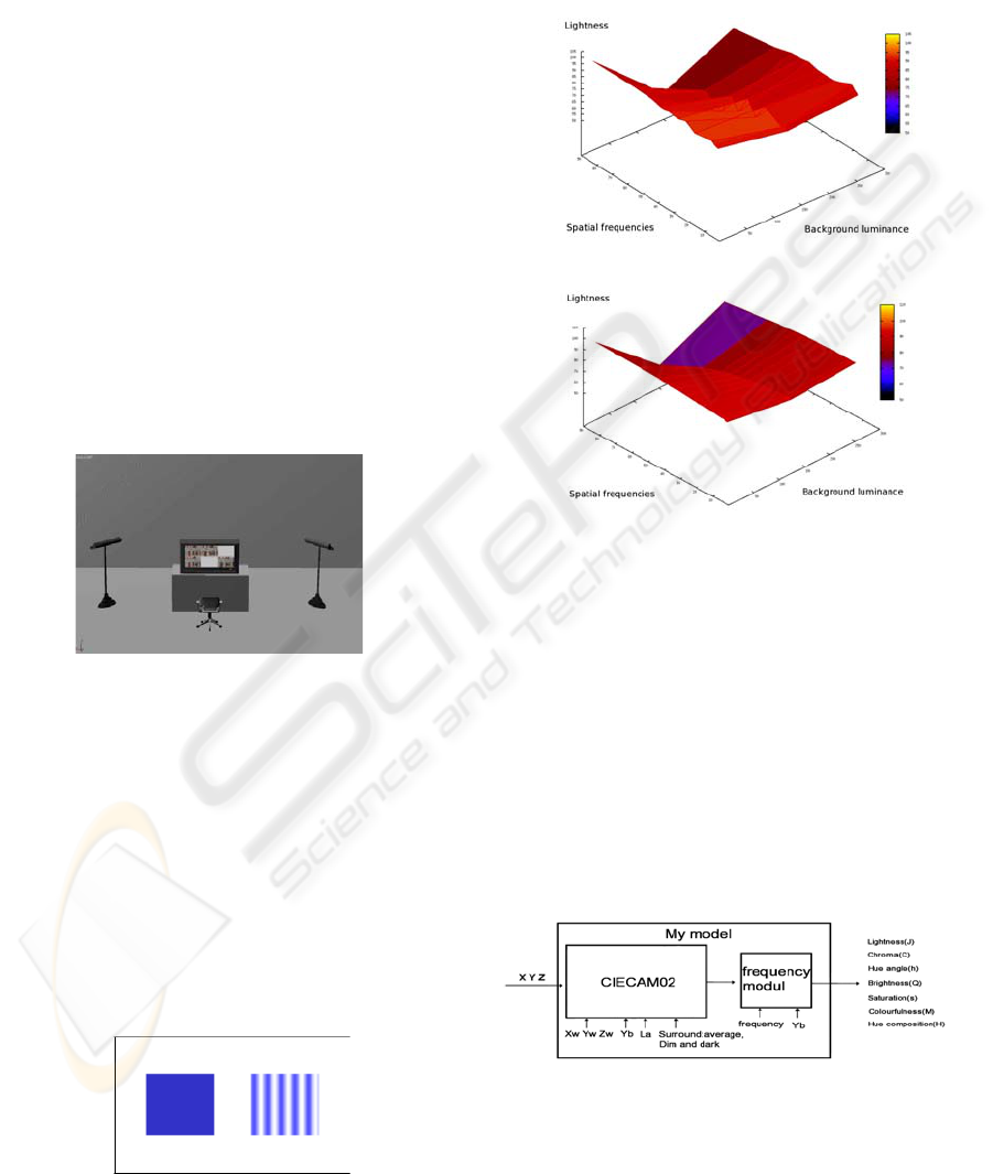
Figure 1: Psychophysical test room.
With regards the recommendations given by
standards ISO 3664 (ISO3664 2005) and ITU-R
500-10 (ITU-R Recommendation 2000) this
environment should respect many conditions as for
example the color of walls which should be neutral
or the background chromaticity which should
correspond to the illuminant D65.
The experiment realized was based on the
adjustment of the hue angle, the lightness and the
chroma of the stimuli in order to appear similar to
the input color. The figure 2 gives a snapshot of the
tests run for blue stimulus.
Figure 2: Example of test pattern.
Thanks to this test, the influence of the spatial
frequency on our perception has been measured for
several frequencies on three different achromatic
backgrounds with different luminance.
The figure 3 illustrates the results obtained for the
red lightness.
-a-
-b-
Figure 3: Results for red lightness: a-measured, b-
modeled.
The obtained results from the described experiments
represent the difference perceived on the hue angle,
the lightness and the chroma according to the spatial
frequency and the background luminance.
For modeling the results, curves of degree two were
chosen and have been fitted using the least square
method. An example is given by figure 3-b for the
red lightness.
The figure 4 shows the diagram of the s-CIECAM. It
represents the integration of a spatial module in the
standard CIECAM02
Figure 4: Diagram of input/output of s-CIECAM.
Thus, this model is able to predict all effect
predicted by the CIECAM02 in addition to the
spatial adaptation.
USE OF SPATIAL ADAPTATION FOR IMAGE RENDERING BASED ON AN EXTENSION OF THE CIECAM02
129
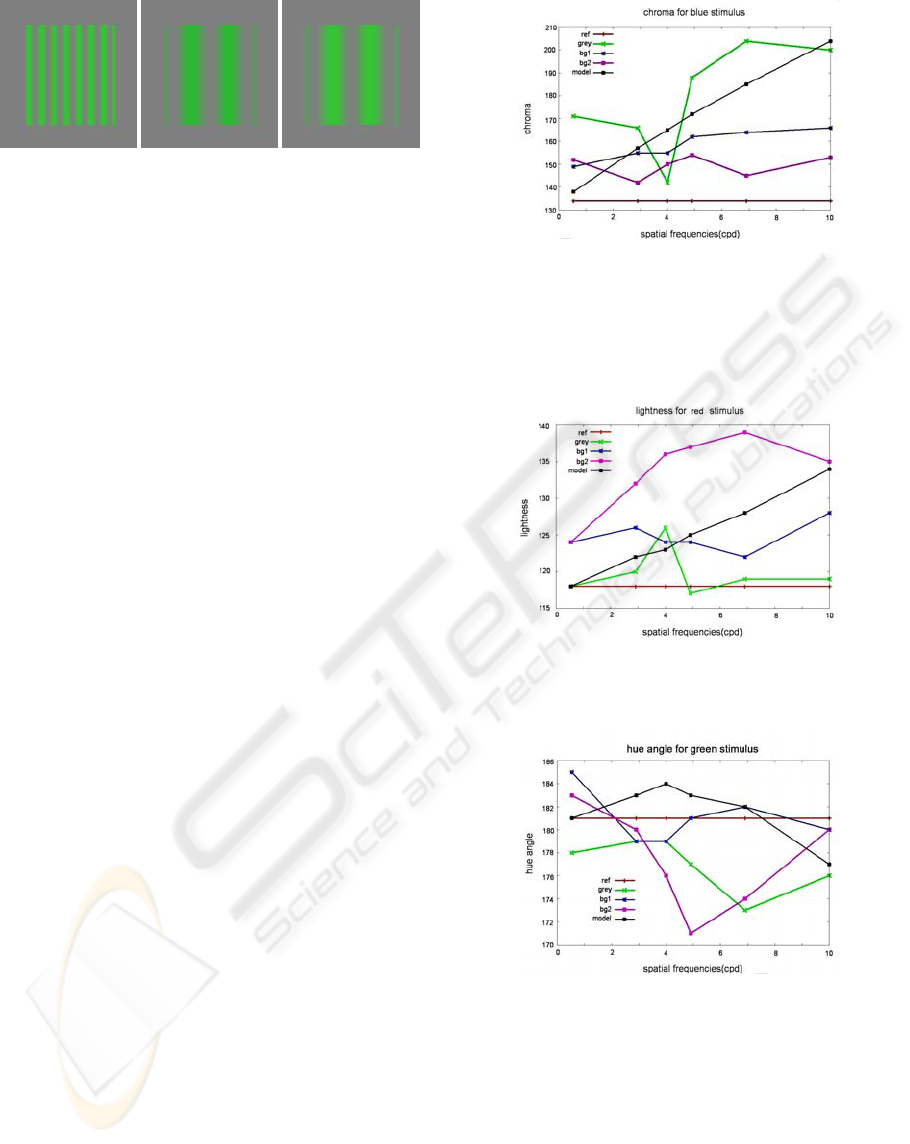
-a- -b- -c-
Figure 5: Example of corrected pattern. a- input stimulus
at frequency f. b- stimulus at frequency f’ and same color
as (a). c- Spatially corrected stimulus from f to f’.
In figure 5, an example of correction for a green
stimulus on a grey background is given. The input
stimulus is at a given frequency f. When this
frequency is decreased to f’, we obtain the stimulus
of figure 5-b. It is easy to notice that the two colors
seem different. By using the s-CIECAM, for the
spatial correction, the corrected stimuli (figure 5-c)
are closer to the input one.
Even if the obtained results are quite encouraging,
the s-CIECAM is designed to correct only one
stimulus and is not adapted to the correction of
images.
2.1 Influence of Background’s
Chromaticity
At this stage, the S-CIECAM is only taking into
account the frequency and of the background
luminance. New experiments have been conducted
in order to study the influence of background’s
chromaticity on human perception. In these
experiments, the background of a stimulus is no
longer achromatic but really chromatic.
The preparation and the conduction of subjective
experiments are tedious and time consuming. Our
selection of background has lead to two colors
having same luminance as the grey used in
precedent campaign to have a maximum of different
chromaticity with the same luminance.
Thus the perceived difference between a flat
stimulus and a stimulus modulated by a spatial
frequency, on three different backgrounds which
have the same luminance , is measured on the three
perceptual components J, C and h. An example of
results is shown by the figures 6, 7, 8:
Figure 6: Average of chroma perceived on a blue pattern,
on different backgrounds with the same luminance on
several frequencies (ref : reference color, grey :
achromatic background, bg1: 1st chromatic background,
bg2: 2nd chromatic background and model: s-CIECAM
predicted values).
Figure 7: Average of lightness perceived on a red pattern,
on different backgrounds with the same luminance on
several frequencies (same labels than figure 6).
Figure 8: Average of hue angle perceived on a green
pattern, on different backgrounds with the same luminance
on several frequencies (same labels than figure 6).
The obtained results show that the perceived
differences are quite similar for the hue angle and
the lightness comparatively to their scale. But the
figure 7 presents an important gap in the chroma for
high frequencies.
These figures show also that the s-CIECAM model
has a sound prediction of the spatial effect related
for the hue angle and the lightness.
VISAPP 2008 - International Conference on Computer Vision Theory and Applications
130
3 IMAGE APPLICATION
In order to use this spatial model for image
rendering, an extension was necessary because the
S-CIECAM is able to correct single stimuli only.
3.1 Model Description
It is very important to deal with image correction
since it is the main material we use in different
applications. The extension of the s-CIECAM to
images is not obvious. Indeed, the image is
composed by pixels where each of them could be
considered as a stimulus. Moreover, there is a
different meaning to be given to background
luminance, to surround and so on.
Starting from these remarks, we have to retrieve
for each pixel its inherent frequency and its
background.
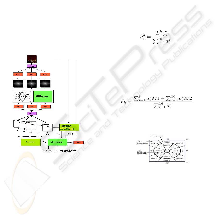
Figure 9: Flowchart of the images s-CIECAM.
The approach that we have adopted could be
summarized by figure 9. The input image is
transposed in the XYZ color space and then in the
Fourier domain. After that, the Fourier space is
decomposed in 17 frequency bands as shown in
figure 10. It corresponds to low, medium and high
frequencies and 8 major orientations.
As a first step, the low frequencies are removed
from the frequency domain in order to preserve the
quality of the image. The other zones with higher
frequencies will be processed using a methodology
that will be discussed hereafter.
• For each of the 16 frequency bands, an
average value is defined based on the size of
the picture and the distance between the
display and the observer.
• Then the inverse Fourier transform is applied
separately for each of these frequency bands
to obtain 16 different pictures representing
the content of each band with the dedicated
frequency and orientation.
For example, the first zone gives an image which
has a high correlation with horizontal medium
frequencies whereas the 11th zone gives an image
with a high correlation with high vertical
frequencies.
For each pixel and for each component (J, C and
h), 16 coefficients are calculated in function of the
frequency band like describe by the equation 1:
(1)
where k represents the perceptual component (J,
C or h) and the B
k
(i) are the value of the component
k at the considered point, for the frequency band i.
These coefficients will be used after to balance
the background luminance and the average
frequency of the pixel area.
The equation 2 describes how a component
frequency is obtained for a given pixel.
(2)
where M1 and M2 are the average frequencies of
the medium and the high frequencies computed
using the image size and the distance
display/observer.
Figure 10: Decomposition in Fourier domain.
The final frequency F is obtained with an
average of the three frequencies F
J
, F
C
and F
h
.
At this stage, for each pixel we have determined a
spatial frequency that could be used directly to
correct it using the s-CIECAM. However, we need
to know the other inputs of this model such as the
background luminance that depends on the
neighborhood of this pixel. The other inputs are
considered as fixed values because they are common
to the whole pixels of the image. It concerns the
tristimulus values of the source white in the source
conditions (X
w
Y
w
Z
w
), the luminance of the adapting
USE OF SPATIAL ADAPTATION FOR IMAGE RENDERING BASED ON AN EXTENSION OF THE CIECAM02
131
field (L
a
) and the viewing conditions (F
l
,c,n
c
).
As the same manner to the frequency, a
background luminance is calculated for each pixel
and the same coefficients a
k
balance the value of the
background luminance. This value is taken directly
from the input image and is depending on the
orientation of the considered neighborhood like
shows the figure 11.
Figure 11: The pixel (in red) and its neighborhood
function of processed band.
For example, in the first area there is a high
correlation with the horizontal frequencies. So, to
specify a background luminance, the pixels which
are above and below are considered for the
computation. If the average luminance of the pixels
above the processed one is close to its luminance,
the average luminance of the pixels below is
considered as the background luminance. If the two
averages are very different from the processed pixel,
the background luminance is considered as their
medium value.
After the background luminance computation, we
can consider that we have the necessary inputs for s-
CIECAM in order to correct the image appearance.
So the first step will be to transpose each pixel into
the perceptual color space composed by the
lightness, the chroma and the hue angle. Then, from
the perceived values for each pixel, it is possible to
apply the inverse s-CIECAM to obtain the corrected
pixel with regards to the input values depending on
varying viewing conditions
In order to obtain a better image and so to validate
the advantages of this proposed approach, we opted
for varying the spatial frequency only. To do that,
the input pixel is considered as belonging to a flat
stimulus at zero-frequency and the inverse model is
used with the frequency obtained by equation1.
3.2 Results
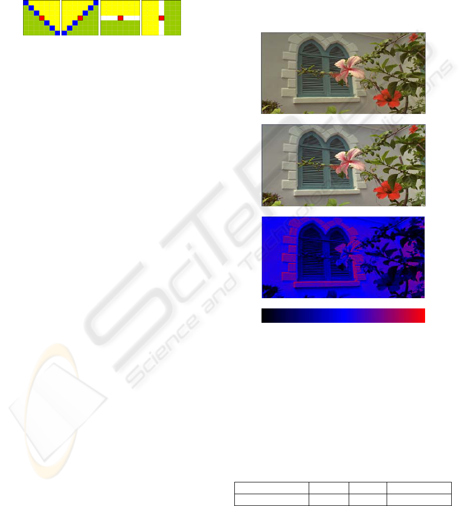
The figure 12 shows an example of the obtained
results using the s-CIECAM adapted to images. In
this figure, we can compare the original picture
(figure 12-a) and its correction with our model
(figure 12-b). It is easy to notice that the corrected
image seems more natural than the original one.
We have done a lot of tests in order to quantify
the improvement done by our approach. Among the
tests, we have performed a similarity measurement
between the original and the corrected images using
the SSIM (Wang, Bovik, Sheikh, and Simoncelli
2004) metric that evaluate the fidelity of the
reproduction. Table 1 gives the fidelity values for
the image of figure 12.
The model has been applied on 17 images
coming from the Kodak image database and the
fidelity between the corrected and the original
images is always high. The CIE ∆E2000 (Sharma,
Wu, Dalal 2005) was also used and the results are
similar to SSIM.
-a-
-b-
-c-
-d-
Figure 12: Example of results. a- original picture. b-
Picture corrected.c-∆E2000 differences between a and b.
d-∆E2000 scale increasing from black to red.
The Figure 12-c shows the error generated by the
correction using the CIE ∆E2000. In this figure,
black represents unmodified pixel, blue represents
zones with a medium difference and red zones have
higher differences.
Table 1: Fidelity measures between original and corrected
images of figure 12 on the three components RGB.
Component Red Green Blue
Fidelity 99.5% 99.4% 97.9%
VISAPP 2008 - International Conference on Computer Vision Theory and Applications
132
From this figure, one can remark that the
textured areas are corrected whereas the relatively
uniform zones.
Another statistical measure has been performed
to prove the consistency of our method which is not
only based on lightness adjustment. Table 2 gives
the average adjustment performed on the 3
perceptual components (J, C and h) for the image of
figure 12.
The values of this table demonstrate that not
only lightness is adjusted but also the chroma and
the hue even if for this latter the deviations are
small.
Table 2: Average adjustment values obtained from the
corrected image of figure 12.
Component J C h
Average adjustment 2.64 9.25 0.05
3.3 Validation
In order to validate our adaptation of s-CIECAM to
images, we have managed a psychophysical
experiments based on a forced choice paradigm.
These subjective experiments were performed on 17
images from the Kodak database. They were
performed with a panel of 15 observers which were
evaluated for the visual acuity and a normal color
vision.
The observers were only asked to choose the
image that seems to them better (more natural)
between an original and a corrected image in a blind
way. Three repetitions are made for each of the 17
pictures to see if the observer has a stable opinion.
The obtained results are presented by figure 13
which shows number of choice of corrected image
against original.
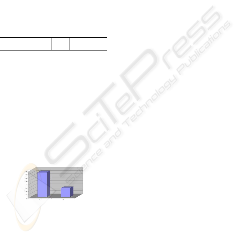
Figure 13: Diagram which show the percentage of choice
for the corrected image (1) against the original (2).
On this histogram we can see that in 75% of case the
image corrected by our model was preferred by the
observers.
The standard deviation is very weak and no
observers have been rejected because of the stable
evaluation they have given.
4 CONCLUSIONS
In this contribution a model based on
psychophysical experiments has been described. A
study of the influence of the chromaticity of the
background was realized with the same experiment.
This s-CIECAM was extended to images with a
method allowing taking into account spatial
information.
Different tests to validate our results were
presented and corrected pictures seem more
naturally than the original. Those results are very
encouraging and the future direction of this work is
its inclusion for High Dynamic Range rendering.
Finally another prospect is the study and the
integration of the temporal frequencies with digital
cinema as an application.
REFERENCES
M.D.Fairchild, “Color appearance model”. Addison-
Wesley, Massachussets (1997).
N. Moroney, M.D. Fairchild, R.W.G. Hunt, C.J Li, M.R.
Luo, and T. Newman, "The CIECAM02 color
appearance model," IS&T/SID 10th Color Imaging
Conference, Scottsdale, 23-27 (2002).
ITU-R Recommendation BT.500-10, “Methodology for
the subjective assessment of the quality of television
pictures “, ITU, Switzerland (2000).
ISO3664, “Viewing Conditions for Graphic Technology
and Photography”, ISO (1999).
M.R. Luo and R.W.G. Hunt, "The Structure of the CIE
1997 Colour Appearance Model (CIECAM97s),"
Color Res. Appl., 23, (1997).
G.M. Johnson, “The quality of appearance”, AIC 2005,
Granada Spain, (2005).
B.A. Wandell “Foundations of vision”, Sinauer
Associates, Inc, Sunderland, Massachussetts(1995).
C. Larabi and O. Tulet, “Study of the influence of
background on colour appearance of spatially
modulated patterns”, CIE, Paris(2006)
G. Sharma, W. Wu, E. N. Dalal, “The CIEDE2000 Color
difference Formula: Implementation Notes,
Supplementary Test Data, and Mathematical
Observations,” CR&A, 30(1), pp. 21-30, 2005.
M.D. Fairchild and G.M. Johnson, “The iCAM framework
for image appearance, differences, and quality,”
Journal JEI 13, 126-138 (2004).
Z. Wang, A. C. Bovik, H. R. Sheikh, and E. P. Simoncelli,
“Image quality assessment: From error visibility to
structural similarity”, IEEE TIP 13 pp.600-612, Apr.
2004.
USE OF SPATIAL ADAPTATION FOR IMAGE RENDERING BASED ON AN EXTENSION OF THE CIECAM02
133
