MULTI-ERROR CORRECTION OF IMAGE FORMING SYSTEMS
BY TRAINING SAMPLES MAINTAINING COLORS
Gerald Krell and Bernd Michaelis
Otto von Guericke University Magdeburg, PO Box 4120, 39106 Magdeburg, Germany
Keywords:
Image restoration, image deconvolution, color processing, color constancy.
Abstract:
Optical and electronic components of image forming devices degrade objective and subjective quality of the
acquired or reproduced images. Classical restoration techniques usually require an explicit estimation or
measurement of parameters for each error source. We propose to derive restoration parameters in a training
phase with suitable test patterns for a particular system to be corrected. Space varying properties of different
classes of image degradations are considered simultaneously. It is shown how training is performed in such a
way that colors are reproduced correctly independently of the used test patterns.
1 INTRODUCTION
Whereas enhancement algorithms mostly seek to im-
prove subjective image quality (e.g.(Kober et al.,
2003)), image restoration algorithms aim to deter-
mine an image which is as similar to the original as
possible (e.g.(Berriel et al., 1983)). Many approaches
to image restoration and enhancement often consider
a certain image with its degradations and then try to
find correction parameters for this particular image.
We use a training procedure instead with suitable test
patterns in order to compensate defect mechanisms of
the image forming system. This enables us to design a
powerful correction system for the simultaneous com-
pensation of several image defects. Training data are
selected and modified carefully and the training is ap-
plied in such a way that the behavior of the applied
color model can be controlled in a deterministic way.
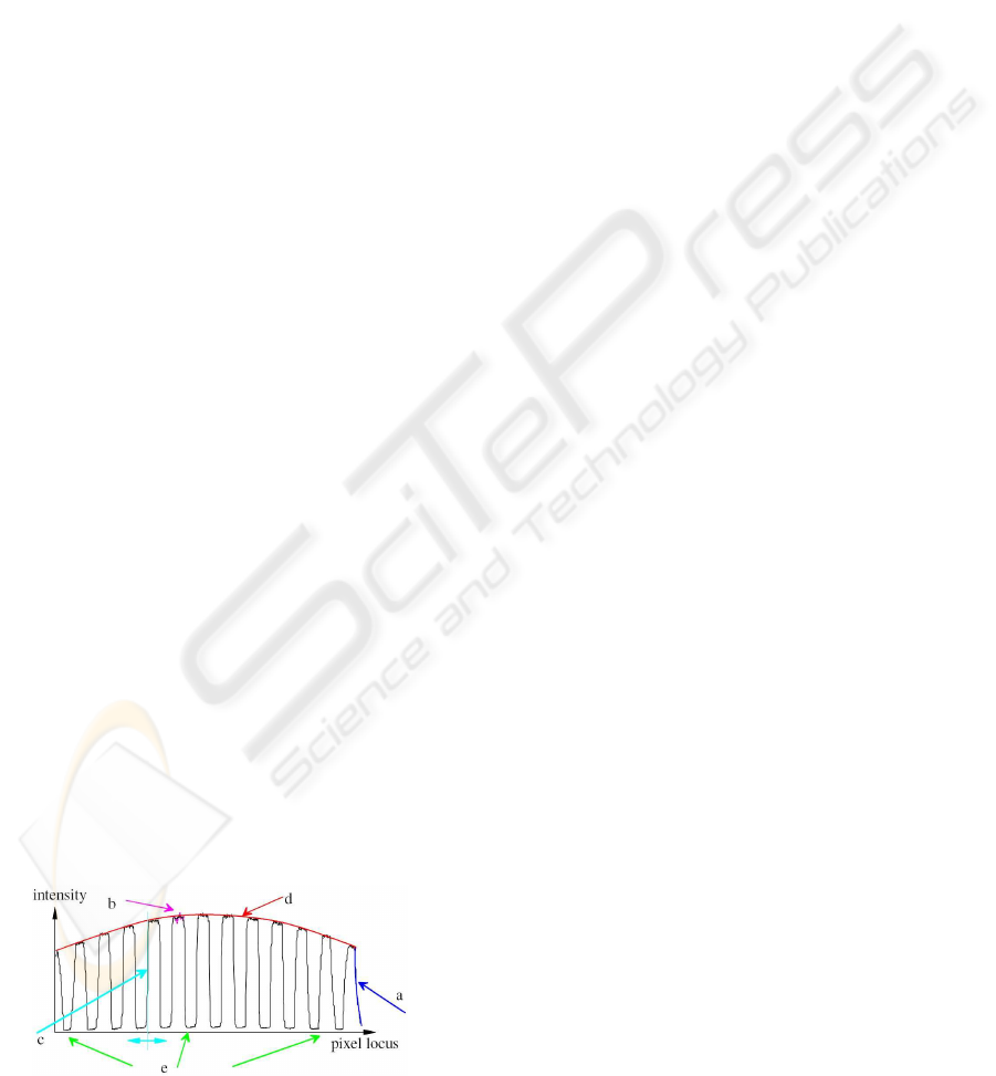
Typical image defects are shown in Fig. 1. For
simplicity the image of a black and white line camera
is shown.
Figure 1: Typical types of image degradation demonstrated
with an image of a regular grating captured by a line camera.
Typical image defects to be considered by the pro-
posed correction technique include (see Fig. 1 for re-
ferring letters)
a blur: caused by defraction limitations or misfo-
cussing of lens
b noise: caused by optical sensor electronics and
image digitization
c geometric distortion: deformation by lens system
d vignetation: shading of lens or display
e space variance: errors usually increase with dis-
tance from optical axis
These effectsusually occur simultaneously and space-
varying. In multichannel systems as used in color
imaging, additional errors occur. We distinguish be-
tween static and dynamic color errors in this paper.
Different blur and distortion properties of the image
channels lead to color divergence in the images re-
sulting in smeared color transition at edges. Fig. 2
shows such errors by a 2-dimensional color image of
a black object on white background: the edges have
a smeared color transition. We call such effects dy-
namic color errors, here.
Errors and limitations of the color model induc-
ing a wrong reproduction of colors even in flat im-
age regions are static color errors. To maintain colors
means in the optimal case that a certain color is re-
produced with the same value by the image forming
system. Many investigations have been undertaken in
the field of color constancy, where the main focus is
152
Krell G. and Michaelis B. (2008).
MULTI-ERROR CORRECTION OF IMAGE FORMING SYSTEMS BY TRAINING SAMPLES MAINTAINING COLORS.
In Proceedings of the Third International Conference on Computer Vision Theory and Applications, pages 152-158
DOI: 10.5220/0001084401520158
Copyright
c
SciTePress

a
b
Figure 2: Color divergence as a typical defect in multichan-
nel image systems: a) ideal convergence; b) edge smearing
caused by color divergence.
the estimation of the color of object in images with an
illumination by light of unknown color characteristics
((Barnard et al., 1997; Kobus, 2002; Verges-Llahi and
Sanfeliu, 2003; Ebner, 2003)). In this paper we con-
sider how the restoration system is trained by suitable
test patterns. Normally, additional constraints must
be introduced to avoid a too strong dependence of the
correction result on the selected test patterns. Oth-
erwise a correct color reproduction for random input
images is not given. It is clear that the restorations
system must not induce additional color errors, but if
required it should compensate color errors of the im-
age forming system instead.
In many investigations of image restoration (Gon-
zalez and Woods, 1993; Andrews, 1977; Zheng
and Hellwich, 2007) the process of image formation
and restoration is treated by a system as shown in
Fig. 3. We generalize the considerations for a multi-
dimensional system with continuous coordinates~x =
x
1
... x
K
T
and C channels (e.g. colors). This
scheme is very similar to approaches in system the-
ory (Unbehauen, 1970; K¨upfm¨uller, 1949). (Jahn and
Reulke, 1995) applies system theory directly to opti-
cal sensors. As an initial assumption, the characteris-
f(~x)
ˆ
f(~x)
g(~x)
n(~x)
h(~x,
~
ξ) w(~x,
~
ξ)
Figure 3: Basic model of image forming and restoration.
tics of the correction system are opposite or ”inverse”
to those of the degrading system - provided the cor-
rected image approximates the input image as far as
possible. Such inverse problems are in general ”ill-
posed”. In traditional designs, additional constraints
for a reasonable and stable solution are introduced
(Gonzalez and Woods, 1993). Well- known image
restoration techniques such as the Wiener or Inverse
Filtering methods are available (Stearns and Hush,
1999). Such techniques estimating optimal correc-
tion systems are also called deconvolution (Gull and
Daniell, 1978; Andrews, 1977; Zheng and Hellwich,
2007). However, deconvolution requires knowledge
of system parameters such as noise impact or point
spread function that have to be measured or estimated
in advance. Furthermore, other image degradations,
namely, geometrical distortions, space-varianceof pa-
rameters and unknown errors require additional cor-
rection methods.
In a K-dimensional
1
image forming system with C
channels (colors for instance), channel c has the illu-
mination distribution g
c
(~x) resulting by summing up
the K-ply integrals of the object illumination distri-
bution channels f
c
(~x) above the pulse response of the
the image formation system between channels c and
q, h
c,q
(~x,
~
ξ), also called cross point spread function
(PSF), and superposition with channel specific noise
function n
c
(~x):
g
c
(~x) =
C
∑
q=1
∞
R
−∞
.. .
∞
R
−∞
h
c,q
~x,
~
ξ
f
q
~
ξ
dξ
0
.. . dξ
K−1
+ n
c
(~x)
(1)
with
~x =
x
1
... x
K
T
the vector of continuous
coordinates. The continuous vector of local coor-
dinates
~
ξ =
ξ
1
... ξ
K
T
enables us to model
space variance of the PSF. Geometric distortions are
usually modeled by coordinate transforms and also
covered by Eq. 1.
This equation changes to a simple convolution if
the pulse response of the system to be corrected can be
considered stationary (space invariant, see (Andrews,
1977)). (Andrews, 1977) defines image restoration as
to determine the original object distribution f given
the recorded image g and knowledge about the point-
spread-function h. Approaches that compensate for
a convolution of the original by the PSF are often
called image deconvolution (Gonzalez and Woods,
1993; Andrews, 1977). The task of image restoration
requires therefore the determination of a system with
the pulse response w(~x,
~
ξ) which produces an output
ˆ
f(~x) approximating the input f(~x).
Considering pixel-based image forming devices
with images of limited extent leads to a discrete, alge-
braic representation of the system which is shown in
Fig. 4a). Multi-dimensional image data is vectorized
to form image vectors . The length of these vectors is
the product of numbers of pixels in each dimension by
the number of channels. As an example, let us con-
sider the pixel values of an original image f
l
1
,···,l
K
,c
where l
1
···l
K
are the pixel indexes in the K dimen-
sions and c is the index of the image channel. This
image is described by object vector
~
f which is ob-
tained by vectorization of the input image pixels in
1
We generalize our approach for multidimensional im-
age systems with any number of channels
MULTI-ERROR CORRECTION OF IMAGE FORMING SYSTEMS BY TRAINING SAMPLES MAINTAINING
COLORS
153

each dimension and each channel as:
~
f =
f
1,···,1
··· f
D
1
,···,D
K
,1
··· f
D
1
,···,D
K
,C
T
.
D
1
···D
K
are the image extents in the K dimensions
andC the channel number. Noise superposition vector
~n and restoration vector
~
ˆ
f yield by vectorization in the
same way.
This kind of image restoration model is often sub-
ject of so called optimal restoration approaches (e.g.
(Jain, 1998; Katsaggelos, 1999)). Such techniques
usually seek a trade-off between noise suppression
and sharpening in the restored image vector
~
ˆ
f.
~
H and
~
W describe the point spread function matrices of the
image forming and the restoration systems, respec-
tively. With the assumption of perfect compensation,
~
f
~
f
ˆ
~
f
ˆ
~
f
ˆ
~g
~g
~
W~n
~n
a)
b)
~
H
~
H
~
W
~
W
Figure 4: Restoration of image acquisition (a) and repro-
duction (b).
the systems
~
H and
~
W can change their position in the
processing chain (Fig. 4b) which corresponds to the
situation of an image reproduction system like a dis-
play or printer In this case, not the restored image ap-
pears at the output of the restoration system
~
W but
an image
ˆ
~g with degradations tending to compensate
those induced by the image forming system
~
H.
Linearity is an important prerequisite if linear fil-
tering should be applied correctly. Especially the
Gamma distortion integrated in most systems for ac-
quisition and display must be considered. Often, also
the sensors of CMOS cameras possess a nonlinear re-
sponse in order to allow a high dynamic range of light
intensity. In such cases, often a linear approximation
at the point of operation is possible or a non-linear
correction of the overall system is required.
In both cases of Fig. 4, the remaining devia-
tion
~
ε =
~
f −
~
ˆ
f is the restoration error. With the eu-
clidean norm k
~
εk =
√
~
ε
T
·
~
ε as the dot product of the
transposed and non-transposed deviation vector the
mean-square error is defined MSE =
1
N
k
~
εk
2
, i.e. the
quadratic euclidean norm normalized by the number
N of elements in
~
f or
~
ˆ
f. Generally, other quality cri-
teria are also acceptable, but MSE is easy and reliable
to calculate and in most cases the quadratical criterion
has been proved to correlate very well with subjective
image quality rating .
2 SYSTEM TRAINING
In common restoration approaches, system parame-
ters such as PSF and noise impact are a-priori known
or explicitly measured. This is sometimes cumber-
some and not practical, especially if we consider
space-variant systems. We apply a training method
instead similar to supervised learning of artificial neu-
ral networks (ANN). Here, suitable training and target
patterns are presented to the network. In an learning
phase, the weights of the ANN are optimized in such
a way that a training criterion is matched. ANNs are
widely known in nonlinear image processing appli-
cations, for instance in image segmentation and ob-
ject recognition. Other applications use the adaptive
behavior of ANNs to combine properties of biologi-
cal nerve cells with well known ideas of systems the-
ory (Marko, 1969) or with digital Filters (Flach et al.,
1992). We have a very simple neural model in mind
for modeling the image forming process (see Fig. 5)
which can be applied to technical systems for the im-
age acquisition and reproduction. A similar model
may be also used for the early processing stages in
the retina.
Output pixels
Input pixels
Figure 5: Image forming as a simple neural layer with lat-
eral coupling.
~
f
~
ˆ
f
~g
~n
~
W
~
H
~
ε
Figure 6: Estimation of restoration parameters by adaption.
Applying the aforementioned ideas to the image
forming system Fig. 6 yields. In this example an im-
age acquisition system was considered according to
Fig. 4a. The deviation between the original image
vector
~
f and the restored image vector
~
ˆ
f is assessed
for the adaption of the correction matrix
~
W. As stated
above we assume an image forming system with lin-
VISAPP 2008 - International Conference on Computer Vision Theory and Applications
154

ear behavior in the operating range. This is also mo-
tivated by the demand that the system should work at
different brightness levels in the same manner (super-
position principle). In this case the least mean square
problem is directly treated by solving a linear equa-
tion system for
~
W.
We use L training sample image pairs
~
f
ν
and
~
ˆ
f
ν
each producing a restoration error
~
ε
ν
=
~
f
ν
−
~
ˆ
f
ν
. The
number of training samples should assure that enough
linear independent equations are established to esti-
mate the correction weight matrix
~
W. Test images can
be random patterns to be input to the system, but for
a greater number of parameters in
~
W correspondingly
more test patterns are required what is often too much
effort. Alternatively training data can be thus gained
by taking the pixel data of a neighborhood as sample
data assuming that the system properties in the local
neighborhood is approximately constant. With this
simplification we can train the correction system with
a single test image pair.
The learning objective in the two cases of image
acquisition and reproduction can be formulated for
the whole image and all training samples as:
Q =
L
∑
ν=1
k
~
ε
ν
k ⇒ Min. (2)
that is, the norm of the image error accumulated
for the training data set of size L should be mini-
mized. If we put all training vectors of the train-
ing data set in matrices:
~
F =
~
f
1
···
~
f
L
,
~
ˆ
F =
h
~
ˆ
f
1
···
~
ˆ
f
L
i
we obtain target and recall matrices,
respectively.
The quality criterion Eq. 2 can be separated for
each independent pixel to be corrected or for regions
if constant correction parameters are accepted for that
region. The quality criterion can be stated for each
row number i of the target and recall matrices:
Q
i
=
~
ˆ
F
i
−
~
F
i
⇒ Min. (3)
Because of the vectorized form of the data in the
columns of
~
F and
~
ˆ
F the index i corresponds to a cer-
tain location in the image.
The influence of pixels surrounding a pixel to be
corrected is per se decreasing with increasing distance
(see Fig. 7). Hence the training input data are cut
around a considered pixel forming the learning ma-
trix at a certain location in the image
~
G =
~g
1
··· ~g
j
··· ~g
L
consisting of the training vectors~g
j
resulting by vec-
torization of the couple regions according to Fig. 7
~g
1
~g
C
~
∆
1
~
∆
2
1
2
C
ˆ
f
i
~w
Figure 7: Restoration of one channel component
ˆ
f
i
of one
pixel by correction vector ~w coupling restricted regions
~g
1
.. .~g
C
of the training image channels 1. . .C, in the ex-
ample for a 2-dimensional system (K=2).
i.e. the training vectors are obtained by vectoriza-
tion of the surrounding pixels of all C channels in
the local neighborhood of size ∆
1
∆
2
···∆
K
in the K
dimensions. Hence, the length of each training vec-
tor ~g
j
and weight vector ~w is N = ∆
1
∆
2
···∆
K
C. The
calculation effort for the determination of the weight
vector ~w and for the the calculation of the correc-
tion result (recall) can be considerably reduced if the
multi-dimensional problem is separated for each di-
mension. In this case C weight vectors of lengths
∆
1
···∆
C
are to estimate which is a considerably re-
duced number of parameters N
sep
=
K
∑
k=1
∆
k
C . With
the correction weight vector at a certain location i of
one channel ~w =
w
1,···,1
··· w
∆
1
,···,∆
K
,C
T
and
~
ˆ
i
F = ~w
T
~
G the vector of corrected training pixels (row
i of
~
ˆ
F), Eq. 3 becomes
Q
i
=
~w
T
~
G−
~
F
i
⇒ Min. (4)
The correction weight vector ~w satisfying Eq. 4 is
the least-mean square solution of the equation system
which is overdetermined if L > N (linear independent
training patterns assumed). It can be calculated by
typical least mean square methods, for instance
~w
T
=
~
F
i
~
G
T
inv
~
G
~
G
T
with inv() the inverse matrix operator or more general
~w
T
=
~
F
i
/
~
G (5)
with / the matrix division operator. This holds in the
following considerations analogously.
This looks like a simple solution, but operating
with real images requires some additional consider-
ations. Due to a nonzero black level of real image
forming systems offset parameters o
1
···o
C
should be
included in the compensation system (see Fig. 8).
Otherwise the quality criterion Eq. 4 leads to distor-
tions regarding compensation of the dynamic color
errors: the compensating filters tend to compensate
MULTI-ERROR CORRECTION OF IMAGE FORMING SYSTEMS BY TRAINING SAMPLES MAINTAINING
COLORS
155
~
f
f
1
i
f
2
i
f
C
i
˜
f
1
i
˜
f
2
i
˜
f
C
i
ˆ
f
1
i
ˆ
f
2
i
ˆ
f
C
i
ε
1
ε
2
ε
C
o
1
o
2
o
C
~w
1
~w
2
~w
C
~
W
k
~
W
g
~g
~n
~
H
Figure 8: Estimation of parameters for color transform.
~
f
f
1
i
f
2
i
f
C
i
˜
f
1
i
˜
f
2
i
˜
f
C
i
ˆ
f
1
i
ˆ
f
2
i
ˆ
f
C
i
ε
1
ε
2
ε
C
o
1
o
2
o
C
~w
1
~w
2
~w
C
~
W
−1
k
~g
~n
~
H
Figure 9: Estimation of restoration parameters with color-
adapted training data.
the offset in the image data which leads to over-
shooting and oscillation at edges and other artifacts.
Additionally, real color systems reproduce colors only
with a limited accuracy. The main reason for that
are the absorption curves of the sensor elements in
image acquisition devices or the spectral response of
the pixels of image reproducing devices. These phe-
nomenons lead to a cross coupling between the chan-
nels and can be usually seen as a transformation of
color space. If we want to train the system while con-
sidering color model and offset correctly, we therefore
have to estimate C additional cross coupling parame-
ters and one offset parameter for each color channel
of a C-channel system.
Because human eye is very sensitive to color
changes it is essential to preserve color constancy in
the over-all system. As an example, if the input of
the restoration system is considered correct regarding
the color space the restoration system should not alter
the static colors. That is colors in flat regions should
maintain their values at the output of the correction
system. With this demand, the direct coupling weight
vectors have a sum of 1.0 and the cross coupling vec-
tors a sum value of 0.0. Also the offset value should
be zero to keep the black value as it was. But how
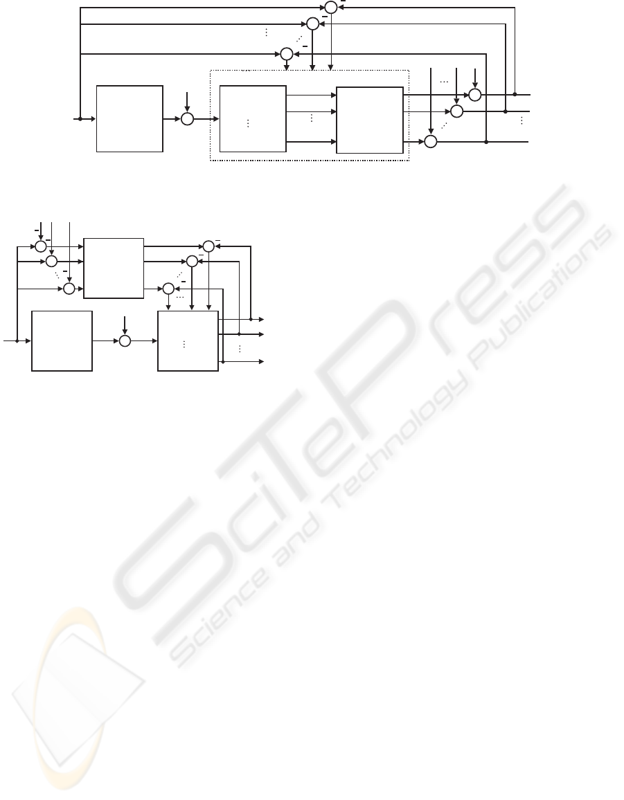
to fulfill this demand? Fig. 8 demonstrates the prob-
lem. It specifies the general system adaption of Fig. 6
for C image channels and introduces offset elements
o
1
···o
C
forming offset vector ~o. The weight vectors
~w
1
···~w
C
together with a coordinate transform matrix
~
W
k
of size C by C establish the general correction ma-
trix
~
W
g
.
~
W
g
and ~o can be directly calculated by the
solution of the equation
~
W
g
~o
~
G
~
1
T
=
~
F
1
i
.
.
.
~
F
C
i
(6)
when
~
F
1
i
···
~
F
C
i
are the selected row vectors of
~
F for
the image channels 1···C at a certain location i sim-
ilar to Eq. 3 and
~
1
T
=
1 ··· 1
is a row vector
of L ones.
In Fig. 8 the matrix
~
W
g
is partitioned in two parts:
the weight vectors ~w
1
···~w
C
and the coordinate trans-
form matrix
~
W
k
. The weight vectors ~w
1
···~w
C
should
only be responsible for the correction of local effects
like blur, color divergence and geometric distortions
(dynamic color errors, see above).
~
W
k
instead should
compensate for intensity related and cross coupling
effects of the image channels (static color errors).
An alternative for the estimation of a correction
system that does not effect static colors is to introduce
constraints in the estimation of
~
W
g
to maintain color
constancy in flat image regions. Such a constraint
could be to claim sums of 1.0 for the main coupling
weight vectors and zero sums for the cross coupling
weight vectors. But investigations have shown that
such a constraint affects the correction of dynamic
color errors and the correction result is unsatisfying.
Therefore another approach is chosen: we adapt
training input and target data so to reflect the same
color coordinate system. Eq. 6 is firstly solved just to
estimate the color rotation between
~
F
i
and
~
G. The pa-
rameters to transform
~
G into the color space of
~
F
i
are
the sums of elements of the direct and cross coupling
weight vectors in
~
W
g
. These sums form
~
W
k
specifying
VISAPP 2008 - International Conference on Computer Vision Theory and Applications
156

the color transform which is applied to
~
F as follows:
~
˜
F
1
i
.
.
.
~
˜
F
C
i
=
~
W
−1
k
~
F
1
i
.
.
.
~
F
C
i
−~o
~
1
T
. (7)
This can be proved assuming that constant colors in
the coupling regions of Fig. 7 are producing the same
value in the restoration pixel (see explanations above
concerning constraints for color constancy). To adapt
the target data
~
F to
~
G we have to subtract the off-
set vector (coordinate translation) and to apply the
inverse of this transformation matrix
~
W
k
(see Fig. 9).
Weight vectors for the correction of dynamic color er-
rors but neutral regarding static color errors can then
be estimated by solving the equation:
~w
1
.
.
.
~w
C
~
G =
~
˜
F
1
i
.
.
.
~
˜
F
C
i
. (8)
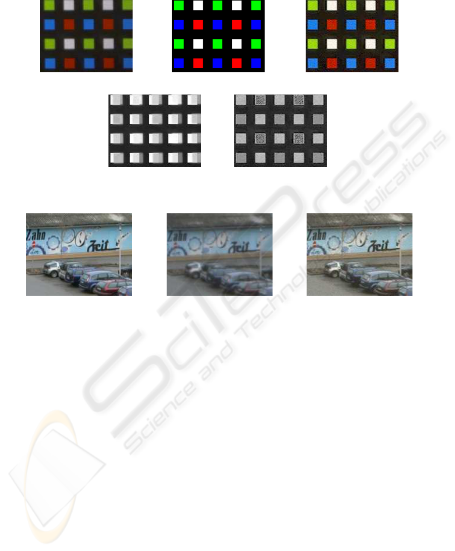
3 RESULTS
In principle, random test patterns for training of the
systems are possible. But the training data set should
reflect all properties of the image errors as much as
possible. We therefore prefer test patterns with maxi-
mal levels of each color and well defined positions of
the edges. As an example a 2-dimensional RGB color
image (C = 3 , K = 2) of checker board type has been
used as input training pattern (Fig. 10b). Such type of
test image assures a sufficient number of linear inde-
pendent input-output relations in the training data.
The image has been displayed by a digital projec-
tion system and captured by a usual digital camera.
The acquired image is shown in Fig. 10a. The result
of training is given in Fig. 10c. Separable weight vec-
tors have been estimated of lengths 30 (∆
1
···∆
3
=
10). Fig. 10d and e show the error of the training
image without and with correction, respectively. The
good compensation of geometric distortions and blur
is obvious. A certain deviation even in the corrected
image remains because of the limited dynamics of
real image forming systems.
As the restoration matrix
~
W is estimated using the
training patterns it can be applied to random data as
long as the degrading system characterized by matrix
~
H doesn’t change very much. This has been done in
Fig. 11. A real-world scene (Fig. 11a) has been dis-
played on the digital projection system and again cap-
tured by a digital camera (Fig. 11b). The correction
result is given in Fig. 11c. This example shows the ap-
plication of the correction method to a combined im-
age acquisition and reproduction system, in this case
consisting of a digital camera and a video projector.
If we assume the camera having a much better im-
age quality than the projections system we can use it
as a restoration system for the latter. We should then
apply the restoration system
~
W to the images to be
displayed.
4 CONCLUSIONS
A teaching approach for the restoration of multi-
channel image forming systems has been proposed.
Several kinds of space-variant errors are treated si-
multaneously and cross-channel effects and offsets
are considered.
The training is based on deterministic test pat-
terns, but the trained system can be applied to random
images. The selection of test patterns is not critical
due to the adaption of the color spaces of input and
target patterns. The required transform matrix is de-
termined in an intermediate step. This avoids the in-
troduction of explicit constraints. The required chan-
nel transform matrix is determined in an intermedi-
ate step. This avoids the introduction of explicit con-
straints. The color transform is estimated correctly
even if training and target regions are not aligned cor-
rectly due to geometric distortions. This way the cor-
rection of the static color model is separated from the
correction of the dynamic errors. This can be impor-
tant for the technical realization of the correction. A
serial connection of a color transform unit and of a
filter processor for each channel can thus be driven
by the estimated parameters. One main benefit of the
proposed approach is the reduction of additional er-
rors, such as geometric distortions and cross chan-
nel errors, that cannot directly be reduced by con-
ventional deconvolution algorithms which are mostly
based on the idea of the Wiener Filter. An explicit
estimation of PSF and noise is not required. By tak-
ing into account the space variant system offset and
cross coupling behavior of real color sensors typical
distortions and color errors are minimized.
REFERENCES
Andrews, H. (1977). Digital Image Restoration. Prentice-
Hall.
Barnard, K., Finlayson, G., and Funt, B. (1997). Color con-
stancy for scenes with varying illumination. Computer
Vision and Image Understanding, 65(2):311–321.
MULTI-ERROR CORRECTION OF IMAGE FORMING SYSTEMS BY TRAINING SAMPLES MAINTAINING
COLORS
157
a
b
c
d
e
Figure 10: Training images: Reproduction (a) Test image (b) Training result (c),(d,e) error images.
a
b
c
Figure 11: Test images (recall): Original (a), reproduction (b), reproduction with correction (c).
Berriel, L. R., Bescos, J., and Santisteban, A. (1983). Image
restoration for a defocused optical system. Applied
Optics, 22, No. 18.
Ebner, M. (2003). Combining white-patch retinex and the
gray world assumption to achieve color constancy for
multiple illuminants. In Pattern Recognition, LNCS
2781, pages 60–66. Springer.
Flach, B., Guth, H., and Osterland, R. (1992). Lokale neu-
ronale filter. In 14. DAGM-Symposium ”Mustererken-
nung”, pages 323–328. Springer, Dresden.
Gonzalez, R. and Woods, R. (1993). Digital Image Process-
ing. Addison-Wesley.
Gull, S. F. and Daniell, G. (1978). Image reconstruction
from noisy and incomplete data. Nature, 272:686–
690.
Jahn, H. and Reulke, R. (1995). Systemtheoretische Grund-
lagen optoelektronischer Sensoren. Akademie Verlag.
Jain, A. (1998). Fundamentals of Digital Image Processing.
Prentice Hall.
Katsaggelos, A. (1999). Digital Image Restoration.
Springer.
Kober, V., Mozerov, M., and Alvarez-Borrego, J. (2003).
Spatially adaptive algorithm for impulse noise re-
moval from color images. In CIARP 2003, pages 171–
179. Springer.
Kobus, B. (2002). Modeling Scene Illumination Colour for
Computer Vision and Image Reproduction: A survey
of computational approaches. Ph.D. thesis, Simon
Fraser University, School of Computing.
K¨upfm¨uller, K. (1949). Die Systemtheorie der elektrischen
Nachrichten¨ubertragung. Hirzel, Stuttgart.
Marko, H. (1969). Die Systemtheorie der homogenen
Schichten. Kybernetik, 5:221–240.
Stearns, S. and Hush, D. (1999). Digitale Verarbeitung
analoger Signale. R.Oldenbourg Verlag, M¨unchen,
Wien.
Unbehauen, R. (1970). Systemtheorie. Akademie-Verlag,
Berlin.
Verges-Llahi, J. and Sanfeliu, A. (2003). A colour con-
stancy algorithm based on the histogram of feasible
colour mappings. In CIARP 2003, pages 171–179.
Springer.
Zheng, H. and Hellwich, O. (2007). Image statistics and lo-
cal spatial conditions for nonstationary blurred image
reconstruction. In Hamprecht, F. A., Schn¨orr, C., and
J¨ahne, B., editors, Pattern Recognition, volume 4713
of LNCS, pages 324–334. Springer.
VISAPP 2008 - International Conference on Computer Vision Theory and Applications
158
