A PDES METHOD PRESERVING BOUNDARIES ON DENSE

DISPARITY MAP RECONSTRUCTION

Ji liu

1,2

, Junjian Peng

1,2

, Yuechao Wang

and Yandong Tang

Graduate University of Chinese Academy of Sciences, Beijing 100039, China

Shenyang Institute of Automation, Chinese Academy of Sciences Shenyang 110016, China

Keywords: Disparity map reconstruction, PDEs, GCPs.

Abstract: Over smoothness restricts the application of PDEs in the field of dense disparity map reconstruction,

because disparity map reconstruction usually requires preserving discontinuousness in some areas such as

the boundaries of objects. To preserve disparity discontinuousness, this paper adopts two strategies. Firstly,

ground control points (GCPs) are introduced as the soft constraint. Secondly, this paper designs a structure

of smoothness part in energy functional, which can preserve discontinuousness effectively. Moreover, the

adjustable parameters in the smoothness part advance its robustness. In experiments, we compare proposed

method with graph cuts method and prove that PDEs is also a useful solution for disparity map

reconstruction and has the advantage of dealing with smooth images.

1 INTRODUCTION

Dense disparity map reconstruction based on two

intensity images is the fundamental research in

stereo vision. It can be described as matching each

point in one image with its correspondent point in

the other one. According to the epipolar constraint,

all possible correspondent points lie in the same line.

Thus, the matching relationship can be described as

the disparity surface D(x,y).

Over the years, numerous algorithms with energy

functional optimization have been investigated in

dense reconstruction via two or more images. In

order to find the best disparity surface, many

researches focus on functional optimization. Graph

cuts and belief propagation, as two discrete

functional optimization methods, have become two

mainstream methods and won academic recognition

(

Marshall and William, 2003). In the field of disparity

map reconstruction, the top contenders for the best

disparity map estimation, on the most common

comparison data, either use belief propagation (Sun

et al., 2003) or graph cuts (Boykov et al., 2001).

Many researches discuss the application of graph

cuts (Roy and Cox, 1998; Birchfield and Tomasi,

1999; Kim et al., 2003) and belief propagation (Sun

et al., 2003; Klaus et al., 2006; Frey et al., 2002;

Felzenszwalb and Huttenlokcher, 2006) in disparity

map reconstruction. Two papers (Kolmogorov and

Zabih, 2004) and (Boykov, 2001) play the important

role in the theory and application of graph cuts. In

(Kolmogorov and Zabih, 2004), the author gives a

precise characterization of what function can be

minimized via graph cuts, and in (Boykov, 2001) the

author introduces two efficient approximation

algorithms to find a local minimum based on graph

cuts. In paper (Sun et al., 2003; Frey et al., 2002;

Felzenszwalb and Huttenlokcher, 2006), the authors

propose some fast and effective approximation

algorithms for belief propagation. Overall, two

methods have been studied broadly and can be

considered as comparatively mature algorithms in

disparity map reconstruction. This paper harvests

considerable profits from their works.

PDEs mothed, as a continuous functional

optimization method, has been applied successfully

in image segmentation (Aubert et al., 2002; Maso et

al., 1992; Kass et al., 1988), 3D reconstruction

(Faugeras and Keriven, 1998; Deriche et al., 1997;

Faugeras and Keriven, 2002), and image recovery

(Aubert and Vese, 1997). However, compared with

graph cuts and belief propagation, PDEs has not

been applied broadly in the disparity map

reconstruction. The PDEs method always assumes

that images can be approximately considered as

continuous functions. Regrettably, the assumption

often can not be satisfied in the disparity map

reconstruction, since the ultimate disparity map

result needs to preserve discontinuousness in some

disparity mutation areas such as the object’s

655

liu J., Peng J., Wang Y. and Tang Y. (2008).

A PDES METHOD PRESERVING BOUNDARIES ON DENSE DISPARITY MAP RECONSTRUCTION.

In Proceedings of the Third International Conference on Computer Vision Theory and Applications, pages 655-661

DOI: 10.5220/0001080606550661

 SciTePress

boundaries. Thus, PDEs method performs very well

in those fields where images are fit to be considered

as continuous function but is not very effective in

disparity map reconstruction. This reason leads to

fewer researches on PDEs application in this field

than graph cuts and belief propagation.

Since PDEs method has its advantage in dealing

continuous situation, this paper still adopts this

method to estimate the disparity map. We hope to

benefit from its advantage and avoid its drawback.

Although we assume that images are continuous

functions, the disparity map calculated via images

can still generate discontinuousness to meet the

expected disparity map. Robert and Deriche (Robert

and Deriche, 1996), in order to preserve

discontinuous boundaries, design the smoothness

function to satisfy that all points should diffuse

mainly in the orthogonal direction of disparity

gradient. Alvarez L. et al. (Alvarez et al., 2000) use

the smoothness function introduced by Nagel and

Engelmann which constrains the diffuse direction

mainly in the colour gradient direction. Their works

are to some extent effective to preserve

discontinuousness and enlighten us a lot.

In order to preserve discontinuities better, this

paper adopts two strategies: ground control points

(GCPs) are applied as the soft constraint conditions

and the image gradient information is introduced to

control the penalty strength in the smoothness

function.

For the former, the ground control points (GCPs)

have two features. Firstly, they usually appear in the

areas where the colour changes suddenly, for

example, the boundaries of objects. Secondly, the

disparity value in GCPs can be gained by some

simple local matching algorithms such as SSD,

ZNCC, and have high reliability. So, proposed

method utilizes the prior information of GCPs to

modify the common cost part of the energy function.

For the latter, the smoothness function serves to

smoothness the disparity surface by penalizing the

variation between neighbour points. However, some

variation should be preserved or not be penalized if

the variation appears on the object boundaries. The

image gradient information is used to distinguish

boundaries or non-boundaries. Thus, we introduce

the image gradient information to control the penalty

strength. To satisfy different images, we design a

general mathematical model for the smoothness

function, which contains several adjustable

parameters for different images.

Finally, according to variational principles, the

Euler-Lagrange equations are deduced. Through

iteratively numerical solving Euler-Lagrange

equations, the disparity map solutions can be

calculated. For lessening the probability of local

minimum, the scale-space approach is utilized as

(Alvarez et al., 2000; Alvarez et al., 1999).

The paper is organized as follows: In Section 2,

we describe how to detect the GCPs. In Section 3,

the energy functional is introduced. The common

cost function will be modified based on the

information of GCPs. We analyze the conditions that

should be satisfied by the smoothness function and

propose a general mathematical model for the

smoothness function. In Section 4, the numerical

schemes of Euler-Lagrange equation and the scale-

space approach are represented. In Section 5, the

experimental results are presented to validate the

GCPs method. This paper ends with a brief

discussion and conclusion in section 6.

2 GCPS

GCPs can provide some more reliable information

for matching. For preserving the boundary

discontinuousness, we want to find out some GCPs

at the Image’s boundaries. This method may be a

little similar as the method in (Kim et al., 2002).

Firstly, all the images are processed by the LOG

filter to generate the new images. Secondly, the new

images are filtered by a defined filter with N

directions as figure 1, which are depicted in (1).

1 sin cos sin cos 1

(, )

xy ifxy

fxy

otherwise

θθ θθ

−

−−<

⎧

⎨

⎩

(1)

To avoid the problem that filters are across the

object boundaries, we perform local matching using

three filters for each orientation, where the centers of

the filters are shifted to the three different positions

as figure 2, and only the best filtering result (the

minimum) is preserved. Thus, each pixel contains N

results. All pixels are classified into two groups

(homogeneous group and heterogeneous group). If

the maximum of the pixel’s N results exceeds a

certain threshold, this pixel is labeled as

heterogeneous pixel; otherwise, it is labeled as

homogeneous pixel. All the GCPs will come from

the heterogeneous pixels. Thirdly, only those pixels

which satisfy the constraint of consistent bi-

directional matching can became GCPs. It is

operated as follows: in the disparity range, each

heterogeneous pixel in the left image is matched

with the pixel in the right image according to ZNCC

measurement. Then, if the best matching pixel in the

right image is a heterogeneous pixel and its best

matching pixel in the left image is consistent, this

pixel can be defined as the GCP and its disparity

value will be recorded.

VISAPP 2008 - International Conference on Computer Vision Theory and Applications

656

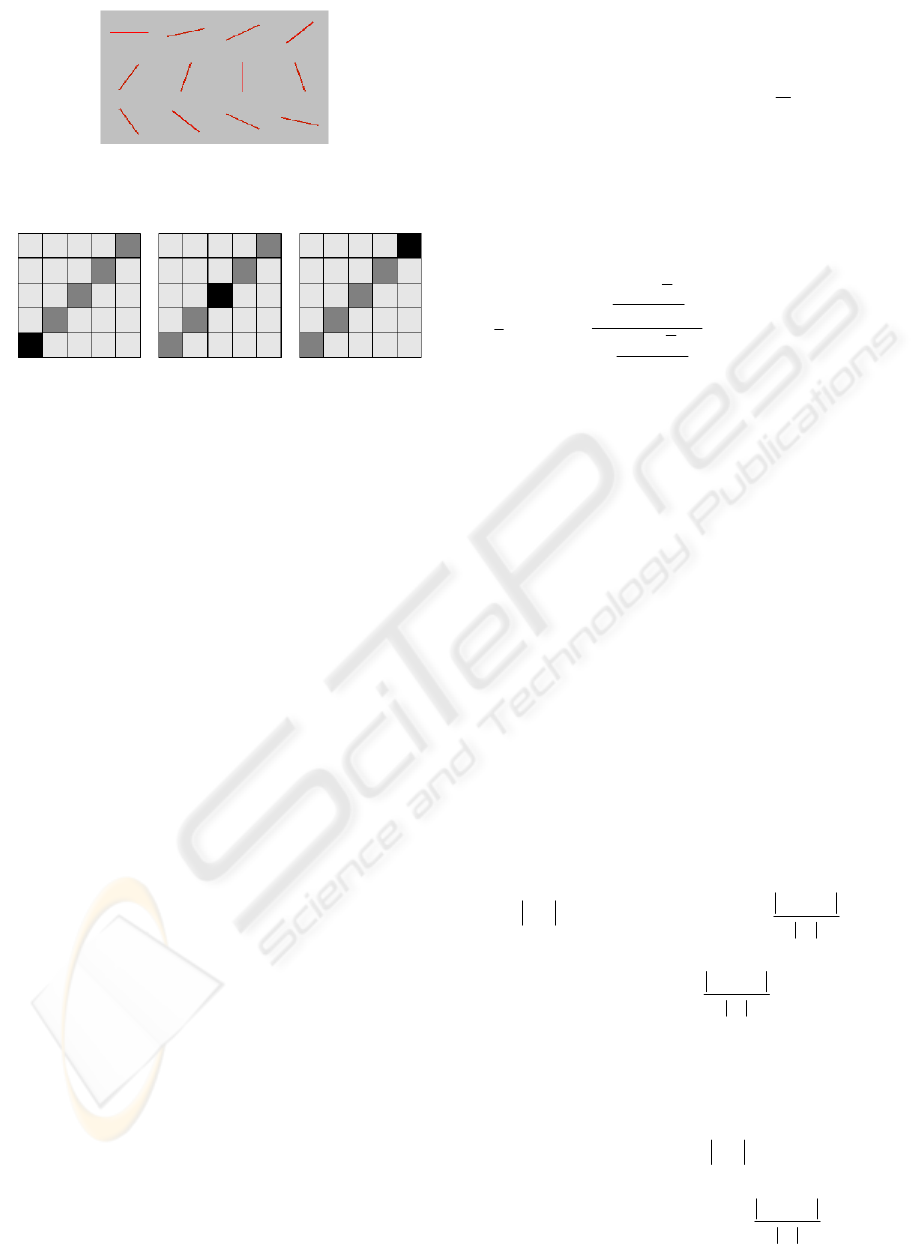
Figure 1: Examples of the rod-shaped oriented filters in

interval of 15

Figure 2: Diagram of the three shiftable oriented filters,

where the centers of the filters are marked in black.

3 THE ENERGY FUNCTIONAL

Generally, the energy function contains two parts in

(2)

() ((,),,) ( (,))ED CDxy xy S Dxy dxdy

=+∇

∫∫

(2)

where the

()C •

is the cost function, the

()S

•

the smoothness function and

Ω is the image

domain.

3.1 The Cost Function

According to the assumption of Lambertian surfaces,

i.e. of objects that look equally bright from all

viewing directions, the two points accurately

matched have the similar intensity in general. Thus,

we define the cost function as follows:

()

(,,) (,) (, (,))CDij Iij I ij Dij=−−

(3)

where

is the intensity in image

=1,2. We

assume two images have been rectified so that the

disparity only appears on the

axis. Equation (3) is

the common frame of the cost part.

However, the expression of equation (3) is

inclined to lead to local minimum. Because it is high

possible that the grey value of one point in left image

is equal to the grey value of more than one points

. Several disparity values of a point may make

the cost part equal to zero. When a certain wrong

value of disparity in one point cause the cost part is

zero, the result may be a local minimum.

In order to reduce the possibility of the local

minimum, we utilize the prior knowledge of GCPs to

flexibly limit the cost function. If a point has been

established as GCPs, the real disparity at this point

should be close to the disparity value

,ij

calculated

during finding out GCPs. The longer the distance

between them is, the larger the cost value is. Thus,

we can design the cost function as (4). The frame

can ensure that only one minimum in GCPs. Thus, to

some extent, the frame can reduce the possibility of

local minimum.

(, )

((,),,)

(, )

((,) (, (,)))

Di j D

ij GCPs

CDijij

Di j D

ij Iij Dij otherwise

⎧

⎛⎞

−

⎪

⎜⎟

⎪

⎝⎠

∈

⎪

⎨

⎛⎞

−

⎪

⎜⎟

⎪

⎝⎠

⎪

−−

⎩

(4)

3.2 The Smoothness Function

The smoothness function is necessary so as to

smooth the disparity surface, since it can be used to

limit the excessive coarseness of the disparity

surface or the discontinuities of

(, )Dxy

. So, it

should be penalized if too large, and the larger the

variation value is, the more the penalty is. However,

the variation at different points should not be

penalized as the same rules. For example, the

variation appearing at the boundary is rational

because we expect it to be discontinuous there, while

the variation appearing at non-boundaries should be

penalized severely. Thus, we utilized the image

information to control the penalty strength and

emphasis.

(, )

∇

represents the smoothness feature of

disparity surface. The penalty

about

(, )Dxy

∇

contains two terms: the penalty

about

∇

and the penalty about

⊥

∇•∇

∇

. The

former means the disparity surface is required to be

as smooth as possible.

⊥

∇•∇

∇

presents the

projection of the gradient disparity in the direction of

the image gradient. So the penalty about it means

that the gradient direction of disparity is supposed to

be consistent with the image gradient direction. If a

point locates in the non-boundary, we more

emphasize the penalty about

∇

in this point than

its disparity gradient direction. If a point locates in

the boundary, the penalty about

⊥

∇•∇

∇

is more

important. The penalty emphasis and strength in a

A PDES METHOD PRESERVING BOUNDARIES ON DENSE DISPARITY MAP RECONSTRUCTION

657

point (

x, y) depends on whether the point is at the

boundary or not. For convenience, we utilize the

image gradient information to sign whether the point

is at the boundary (actually, there is other image

information which can be used to sign the boundary,

and we will discuss them in our future work).

Usually, the boundary is linked with image gradient

module.

Summarily, the smoothness function is described

as this model:

(,) ()( ) ()( )

SDI IS D IS

αβ

⊥

∇•∇

∇∇= ∇ ∇ + ∇

∇

(5)

where

()SD∇

presents the function of

∇

, such

()SD D∇=∇

;

()

⊥

∇•∇

∇

is similar

()SD∇

;

()I

∇

presents the weight of the

penalty of

()SD∇

and

()I

∇

presents the weight

of the penalty of

()

⊥

∇•∇

∇

Estimating

()

∇

and

()

∇

is the key of

estimating the smoothness function. We depict the

constraint conditions of

()

∇

and

()

∇

as below.

Firstly,

()

∇

and

()

∇

must be regularized:

()()1II

αβ

∇+ ∇=

(6)

0>a

(7)

The larger

∇

at a point is, the more probably it

is at the boundary. The opposite is similar. Thus, we

can get:

() ()

aI I if Ib

∇> ∇ ∇<

∇< ∇ ∇>

⎧

⎨

⎩

(8)

where

b is considered as the threshold to estimate

whether the point (

x, y) is at the boundary or not.

Naturally, we can assume

∂

∂∇

∂

∂∇

⎧

⎪

⎨

⎪

⎩

(9)

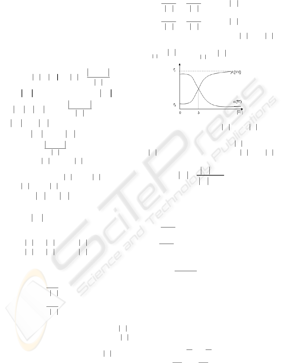
In addition, for decreasing the ambiguousness

near the threshold, we require that the weight

()

∇

rapidly descends at a gradually fast speed while

∇

approaches the threshold from left, and the

descending speed begins to lower while

∇

leaves

the threshold from right. Thus, we add additional

conditions about

and

0, 0

if I b

αβ

⎧

∂∂

>∇<

⎪

∂∇ ∂∇

⎪

⎨

∂∂

⎪

>< ∇>

⎪

∂∇ ∂∇

⎩

(10

)

Based on all conditions above,

()

∇

and

()

∇

can be approximately figured as figure 3, where

lim ( )

∇→

∇

and

lim ( )

∇→∞

∇

Figure 3: Sketchy map of

()

∇

and

()

∇

Then, we define the model of

()

∇

as (11) and

()

∇

can be calculated through

()1()

αβ

∇=− ∇

according to (6).

()

eI f

∇

∇=

∇

(11)

where

e, f, g, and m are constants. According to

conditions (6)-(9), these results are in (12).

⎧

⎪

−

⎪

⎨

−

⎪

−

⎪

−

⎪

⎩

and

0,0 1

mrr><<<

(12)

where

m is decided by the additional conditions (10).

−

and

rr+>

(13)

4 SOLVING EULER-LAGRANGE

EQUATIONS

According to the variational principles, D(x, y) as the

minimum of (1) must fulfill the Euler-Lagrange

equations and boundary conditions:

()0

cos sin 0

DDD

CSS

νν

∂∂

⎧

−

⎪

∂∂

⎪

⎨

∂∂

⎪

∂∂

⎩

(14)

VISAPP 2008 - International Conference on Computer Vision Theory and Applications

658

where

cos

sin

⎡⎤

⎢⎥

⎣⎦

represents a vector normal to the

boundary of

Ω . Equation (14) is solved by the

gradient-descent method or, equivalently, by using a

dynamic scheme as (15)

(, , )

()

cos sin 0

DDD

Dtxy

CSS

txy

νν

∂∂∂

⎧

=− + +

⎪

∂∂∂

⎪

⎨

∂∂

⎪

∂∂

⎩

(15)

where

t is an artificial time.

We discretize the equation by finite differences.

All spatial derivatives are approximated by central

differences, and for the discretization in

t we use

explicit scheme as (16).

( ,,) (,,)

((,,),,)

( ( (,, )) ( (,, )))

Dt ti j Dti j

CDtijij

Dti j Dti j

+Δ −

=−

∂

∂∂

(16)

To avoid the local minimum, a linear scale-space

approach is applied. Typically, we may expect that

the algorithm converges to a local minimum of the

energy functional that is located in the vicinity of the

initial data. To avoid convergence to irrelevant local

minimum, we embed proposed method into a linear

scale-space framework (Robert and Deriche, 2000).

We let

= and

= , where * is the

convolution operator, and

detects a Gaussian

with standard deviation

. We start with a large

initial scale

. Then we compute the disparity

scale

as the asymptotic state of solution using

some initial approximation. Next, we choose a

number of scales:

,(0,1)

σηση

−

=∈

, and we get the

at each

with the initial of

−

. Overall, we

can modify the iterating formation as:

(,,) (,,)

((,,),,)

D t ti j D ti j

CDtijxy

σσ

+Δ −

=−

( ( (,,)) ( (,,)))

D tij D tij

σσ

∂

∂∂

(, )

((,),,)

(, )

( (, ) (, (, )))

iii

Dij D

ij GCPs

C Dij ij

Dij D

ij I ij D ij otherwise

σσσ

⎧

⎛⎞

−

⎪

⎜⎟

⎪

⎝⎠

∈

⎪

⎨

⎛⎞

−

⎪

⎜⎟

⎝⎠

⎪

−−

⎩

(0, , ) ( , , )

ij D ij

σσ

=∞

(17)

5 RESULTS

In this section, we compare proposed method

without considering occlusion with graph cuts

method. All the experiment images come from the

website http://vision.middlebury.edu/stereo. The

images “cloth1” and “cloth3” are contained in the

2006 datasets, the image “Teddy” is in the 2003

database and the image “Tsukuba” is in the 2001

database. In order to evaluate proposed method, the

recognized evaluations (

Scharstein and Szeliski, 2001)

are defined as (18) and (19).

(,)

((,)(,))

R disparityMap x y groundTruth x y

=−

∑

(18)

(,)

((,) (,))

B disparityMap x y groundTruth x y

−>Δ

∑

(19)

where

N is the total number of pixels,

is a

disparity error tolerance. For the experiments in the

paper we use

= . R denotes the average error

value and

B denotes the ratio of the “bad pixels” in

the disparity map. The consequences are showed in

table 1 and figure 4. In the results of proposed

method, the boundaries of objects can be

distinguished clearly. It indicates that the proposed

method owns to the ability of preserving

discontinuousness.

Table 1 presents that the average error value

R in

proposed method is lower than graph cuts method. It

is mainly because that PDEs method has the

characteristic of keeping continuousness. We list the

detail comparison in figure 5. In some continuous

areas, the proposed method can keep the disparity

map continuous better than graph cuts method. The

proportion of “bad pixels” in our method has no

advantage comparing with graph cuts methods,

especially in the image “Tsukuba” with much

discontinuousness. The comparison in “Tsukuba” of

table 1 can reflect this point.

Table 1: Error comparison. The code of GC method comes

from the same website above.

Cloth1

R/B

Cloth3

R/B

Tsukuba

R/B

Teddy

R/B

method

1.015

0.0104

1.766

0.0414

1.247

0.0424

4.9603

0.1317

Proposed

method

0.604

0.0092

0.889

0.0247

0.809

0.0858

1.7703

0.1681

6 CONCLUSIONS

The assumption of continuousness renders PDEs

method difficult to perfectly reconstruct disparity

map. This paper adopts two strategies to preserve

necessary discontinuousness for the disparity map.

The results show that proposed method performs

better than graph cuts method in “Cloth1” and

“Cloth3”, mainly because there images with less

discontinuousness meet the feature of PDEs. The

proposed method can deal with images with much

A PDES METHOD PRESERVING BOUNDARIES ON DENSE DISPARITY MAP RECONSTRUCTION

659

discontinuousness such as “Tsukuba” and “Teddy”

and gain approximate results of graph cuts method.

There are some other aspects which can be

improved. For example, occlusion problem should

be considered, and this problem has exposed in

“Tsukuba” and “Teddy”.

Although it is more difficult for the PDEs

method to preserves boundaries than some discrete

energy methods such as graph cuts method, PDEs

methods have its advantage on keep continuousness.

If we can find some witty strategies to preserve

necessary discontinuousness, PDEs method still can

become a useful solution in disparity map

reconstruction.

REFERENCES

Alvarez, L., Deriche, R., Sanchez, J., Weickert, J., 2000.

Dense disparity map estimation respecting image

discontinuities: a PDE and scale-space based approach.

In Technical Report RR-3874, INRIA.

Alvarez, L., Weickert, J., Sanchez, J., 1999. A scale-space

approach to nonlocal optical flow calculations. In

Scale-Space Theories in Computer Vision, pages 235-

246.

Aubert, G., Barlaud, M., Faugeras, O. and Jehan-Besson,

S., 2002. Image segmentation using active contours:

Calculus of variations or shape gradients? In Research

Report, INRIA.

Aubert, G., Vese, L., 1997. A variational method in image

recovery. In SIAM Journal of Numerical Analysis,

volume 34, pages 1948–1979.

Birchfield, S., Tomasi, C., 1999. Multiway cut for stereo

and motion with slanted surfaces, Proceeding of

International Conference Computer Vision, pages 489-

495.

Boykov, Y., Veksler, O., Zabih R., 2001. Fast approximate

Energy Minimization via Graph Cuts. In Proceeding

IEEE Transaction Pattern Analysis and Machine

Intelligence, volume 23

, pages 1222-1239.

Chan, T. F., Vese, L.A., 2001. Active contours without

edges. In IEEE Transaction on Image Processing,

volume 10, pages 366-277.

Deriche, R., Bouvin, S., Faugeras, O., 1997. A level-set

approach for stereo. In Proceeding SPIE, Investigative

Image Processing, volume 2092, pages 150-161.

Faugeras, O., Keriven, R., 1998. Complete Dense Stereo

vision Using Level Set Methods. In Proceeding

European Conference on Computer Vision, pages 379-

394.

Faugeras, O., Keriven, R., 2002. Variational Principles,

Surface Evolution, PDE's, Level Set Methods and the

Stereo Problem. In IEEE Transaction on Image

Processing, volume

7, pages 336-344.

Felzenszwalb, P. F., Huttenlokcher, D. P., 2004. Efficient

Belief Propagation for Early Vision. In Proceeding

International Journal of Computer Vision, volume 1,

pages 261-268.

Frey B. J., Koetter R., Petrovic N., 2002. Very loopy belief

propagation for unwrapping phase images. In MIT

Press, volume 14.

Kass, M., Witkin, A., Terzopoulos D., 1988. Snakes:

active contour models. In International Journal of

Computer Visiosn, volume 1, pages 321–331.

Kim, J.C., Lee, K.M., Choi, B.T., Lee, S.U., 2005. A dense

stereo matching using two-pass dynamic programming

with generalized ground control points. Proceeding

Computer Vision and Pattern Recognition, pages

1075-1082

Kim, J., Kolmogorov, V., Zabih, R., 2003. Visual

correspondence using energy minimization and mutual

information. In Proceeding International Conference

Computer Vision, pages 1033-1040.

Klaus, A., Sormann, M., Karner, K, 2006. Segment-based

stereo matching using belief propagation and a self-

adapting dissimilarity measure, In International

Conference of Pattern and Recognition, volume 3,

pages 15-18.

Kolmogorov, V., Zabih, R., 2004. What energy functions

can be minimized via graph cuts? In IEEE Trans.

Pattern Analysis and Machine Intelligence, volume 28,

pages 147-159.

Marshall, F. T., William, T. F., 2003. Comparison of

Graph Cuts with Belief Propagation for Stereo, using

Identical MRF Parameters. In Proceedings of the Ninth

IEEE International Conference on Computer Vision,

volume 2, pages 900-906.

Maso, G. D., Morel, J. M., Solimini, S., 1992. A

variational method in image segmentation: existence

and approximation results, In Acta Matematica,

volume 168, pages 89–151.

Osher, S., Sethian, J.A., 1988. Fronts propagating with

curvature dependent. In Journal of Computational

Physics, volume 79, pages 12-49.

Robert, L., Deriche, R., 1996. Dense disparity map

reconstruction: A minimization and regularization

approach which preserves discontinuities. In

Proceeding European Conference on Computer Vision,

pages 439-451.

Roy, S., Cox, I., 1998. A maximum-flow formulation of

the n-camera stereo correspondence problem. In

Proceeding international Conference of Computer

Vision, pages 492-498.

Scharstein, D., Szeliski, R., 2002. A taxonomy and

evaluation of dense two-frame stereo orrespond- dence

algorithms, In International Journal of Computer

Vision, volume 47, pages 7-42.

Sun, J., Zheng, N.N., Shum, H.Y., 2003. Stereo Matching

Using Belief Propagation. In IEEE Trans. Pattern

Analysis and Machine Intelligence, volume 25, pages

787-800.

VISAPP 2008 - International Conference on Computer Vision Theory and Applications

660

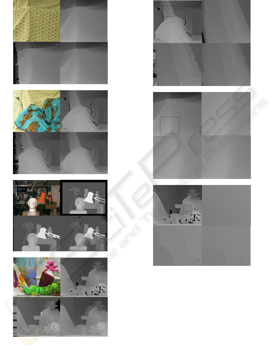
(a)

(b)

(c)

(d)

Figure 4: The disparity map reconstructed by proposed

method and graph cuts. Four group images (a) (b) (c) (d)

respectively are related to Cloth1, Cloth3, Tsukuba and

Teddy. In each group, the left-up, right-up, left-down and

right-down images are respectively left image, ground

truth, the result of GC and the result of proposed method.

(a)

(b)

(c)

Figure 5: The detail comparison of disparity maps. Three

group images (a) (b) (c) respectively are related to Cloth3,

Cloth1 and Teddy. In each group, the left-up, right-up,

left-down and right-down images are respectively ground

truth, local ground truth, local result of GC and local result

of proposed method.

A PDES METHOD PRESERVING BOUNDARIES ON DENSE DISPARITY MAP RECONSTRUCTION

661