
A
FAST AND ROBUST METHOD FOR VOLUMETRIC MRI BRAIN
EXTRACTION
Sami Bourouis and Kamel Hamrouni
Ecole Nationale d’Ing
´
enieurs de Tunis
Laboratoire de Syst
`
emes et de Traitement du Signal : LSTS
ENIT, BP-37, Le Belv
´
ed
`
ere 1002 Tunis, Tunisia
Keywords:
Magnetic Resonance Imaging (MRI), 3D Segmentation, Brain extraction, Expectation Maximization, Level-
set method.
Abstract:
This paper presents a method for magnetic resonance imaging (MRI) segmentation and the extraction of main
brain tissues. The method uses an image processing technique based on level-set approach and EM-algorithm.
The paper describes the main features of the method, and presents experimental results with real volumetric
images in order to evaluate the performance of the method.
1 INTRODUCTION
In brain imaging, image analysis such as segmenta-
tion of anatomical structures is a very important yet
open research problem and is often a first step in the
study of brain anatomy and function. In the context
of neuro-imaging, 3D segmentation of white matter,
gray matter, CSF, etc. is extremely important and has
received much interest in the literature for the recon-
struction, visualization, interpretation of the brain ac-
tivity, and quantitative analysis such as volume mea-
surements. On the other hand, Magnetic Resonance
Imaging (MRI) has become of great interest in many
research areas. This modality allows neuroscientists
to see inside a living human brain, to better localize
specific areas inside the brain and to understand the
relationship between them. However, brain segmenta-
tion and especially the extraction of anatomical struc-
tures from MRI images are a complex problem, be-
cause medical images usually involve a large amount
of data and they sometimes present various artefacts
in the imaging process such as noise, partial volume
effects, intensity inhomogeneities, and because of the
highly convoluted nature of the brain cortex itself.
Thus, it is very difficult to obtain a powerful segmen-
tation tools to be used in clinical routine. This asser-
tion is even more valid in the case of 3D segmentation
of cerebral structures.
In the last several years, many algorithms have
been proposed in this growing area, offering a di-
versity of methods and various evaluation criteria.
For example, several general surveys are reported in
(Pham et al., 1998; Sarang, 2000; Suri et al., 2002).
Shattuck et al. (Shattuck et al., 2001) have developed
a Brain Surface Extraction algorithm (BSE) based
on statistical classification, mathematical morphol-
ogy and connected component operations. In gen-
eral, these methods work efficiently for some segmen-
tation tasks, but partially fail for ”hard cases”. In
addition, there is currently no segmentation method
that provides acceptable results for every type of
medical dataset. 3D brain segmentation using de-
formable model approach is an appropriate frame-
work for merging heterogeneous information and pro-
vides a consistent geometrical representation suitable
for a surface-based analysis. Deformable models are
classified as either parametric active contours or ge-
ometric active contours according to their representa-
tion. Parametric active contours (snakes), originally
proposed by Kass et al. (Kass et al., 1987), are repre-
sented explicitly as parameterized curves. However,
their typical problem consists in its evolution and fi-
nal results are depended on initial shape parameter-
ization. Recently, several attempts have been made
to apply geometric deformable models to brain image
segmentation. In particular, Level-set method (Osher
and Sethian, 1988) is becoming very popular thanks
to its advantages over an explicit representation of
the interface. Indeed, no parametrization is needed,
topology changes are handled automatically, number
461
Bourouis S. and Hamrouni K. (2008).
A FAST AND ROBUST METHOD FOR VOLUMETRIC MRI BRAIN EXTRACTION.
In Proceedings of the Third International Conference on Computer Vision Theory and Applications, pages 461-466
DOI: 10.5220/0001078604610466
Copyright
c
SciTePress
of dimensions is accommodated, and intrinsic geo-
metric properties such as normal and curvature can
be computed easily from the level set function. In
addition, the level-set method has a sub-voxel pre-
cision in its segmentation, a property that very few
segmentation methods provide. An interesting work
on cortex segmentation using deformable models ap-
pears in (Davatzikos and Bryan, 1996) and (Sandor
and Leahy, 1997). Also, Xu et al. (Xu et al., 1999)
have presented a method for reconstructing cortical
surfaces from MR brain images by combining fuzzy
segmentation method, an isosurface algorithm, and a
deformable surface model. In recent studies, several
level set-based methods have been proposed. But, the
problem is that most of these techniques require that
the model should be initialized near the solution or
supervised by an interactive interface. In addition,
computational procedure is another limitation of us-
ing deformable level-set models.
The goal of this work is to provide an automatic
segmentation, based on a level-set deformable model,
for extracting accurately fronts from MR images.
Also, we aim to outline the importance of reducing
processing time in medical image analysis. Like sev-
eral other recent approaches, our design is a success-
ful combination of two approaches, which produces
good results and requires less computing time. Here,
unsupervised classification based on expectation-
maximization (EM) and deformable level-set meth-
ods are integrated into the same pipeline. More pre-
cisely, we apply the EM algorithm and a connected
component analysis on MRI scans to generate inputs
to our deformable model. The synergy between dif-
ferent methodologies tends to result robustness and
optimize processing time that several medical appli-
cations required them.
This paper is organized as follows. In Section II,
we describe our proposed segmentation framework.
In Section III, we present and discuss obtained results
by our framework. Finally, in Section IV, we conclude
our paper and point out future research directions.
2 SEGMENTATION BASED ON
LEVEL-SET APPROACH
Automatic 3D segmentation of the brain from MR
scans is a challenging problem that has received enor-
mous amount of attention lately. Here, we present
our automatic 3D segmentation procedure based on
a deformable level-set method to extract accurately
main tissues from MR images. We notice that a large
number of computations are often needed to solve
the variational equations involved in the Level-Set
model. Nevertheless, good initialization could im-
prove quality results. Furthermore, only few itera-
tions are needed to converge to a sub-pixel accurate
solution. For this reason, we plan to include prior in-
formation about the expected shape. Our proposition
to overcome difficulties consists first on reducing ini-
tial data set to a smaller size. It is an important task in
image analysis that allows overcoming the limitations
of the processing time and become more and more
important, especially, in the case of multidimensional
signal processing. Thus, estimating parameters on the
new sample can be done easily and rapidly.
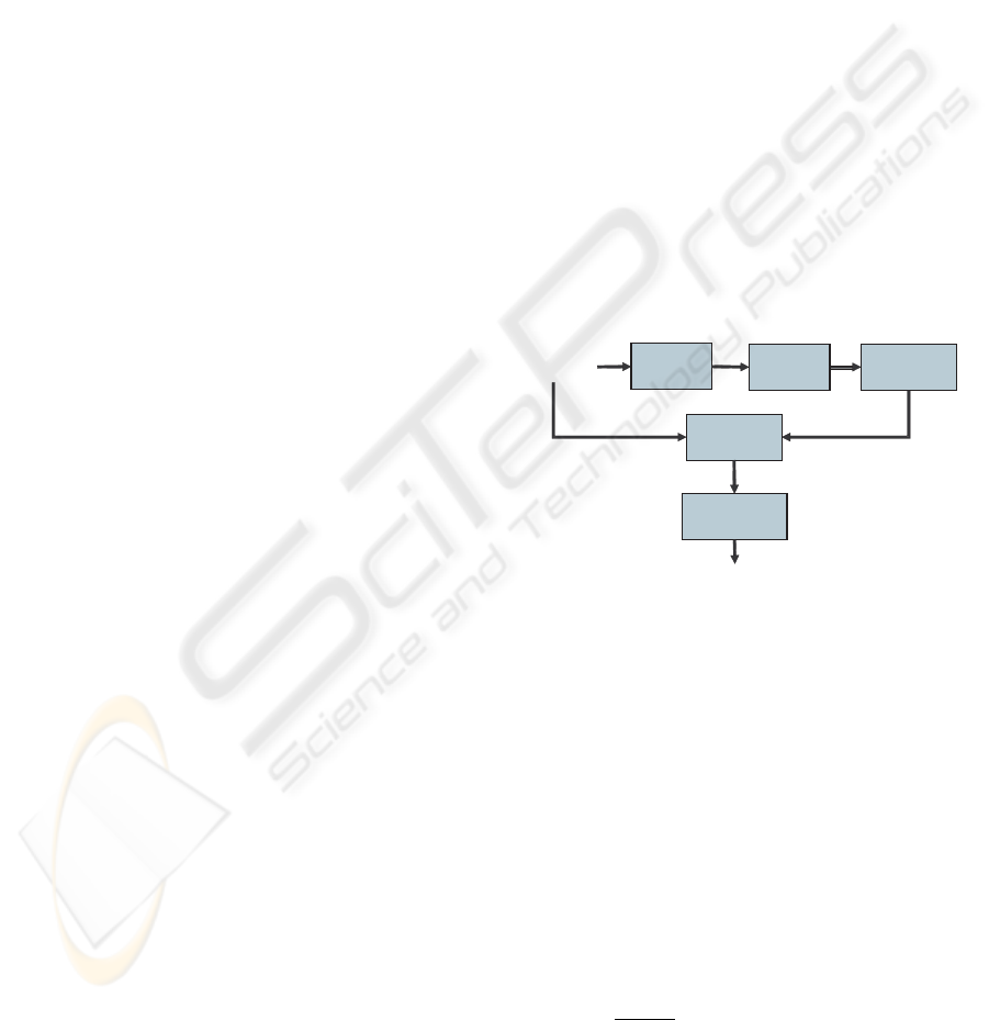
Our brain extraction algorithm uses three stages to
segment image. The first one is the dada smoothing
and the all non-brain tissue removal (i.e. skin, bone,
fat, etc.) from initial data set. In the second stage, we
apply a downsampling process that reduces data size
and furthermore overcomes computation time. The
final stage consists of segmenting, with more preci-
sion, brain structures by using level-set method. Fig-
ure 1 illustrates the major computational steps in the
proposed method.
Volumetric MRI
data
DownSampling
volume
Brain tissues
Estimating
Clustering
Deformable Level-set
model
Reconstructed
surface
Deformable surface
Initialization
Parameters
Preprocessing
Figure 1: General principle of our method.
2.1 Preprocessing Data
Generally, the data volume can contain various
amounts of noise. To eliminate noise, a smoothing
filter is applied (Perona and Malik, 1990). This fil-
ter is supposed to remove only high-frequency noise
and should not affect relevant major geometrical fea-
tures. Authors formulate the anisotropic diffusion fil-
ter as diffusion process that encourages intra-region
smoothing while inhibiting inter-region smoothing.
The diffusion function is given as :
∂I(
¯
X,t)
dt
= ∇(C(
¯
X,t).∇I(
¯
X,t)) (1)
Where, I(
¯
X,t) is the MR image.
¯
X refers to the im-
age axes (i.e. x,y,z ) and t refers to the iteration
step. C(
¯
X,t) is called the diffusion function and is a
VISAPP 2008 - International Conference on Computer Vision Theory and Applications
462
monotonically decreasing function of the image gra-
dient magnitude. It allows for locally adaptive diffu-
sion strengths: edges are selectively smoothed or en-
hanced based on the evaluation of the diffusion func-
tion.
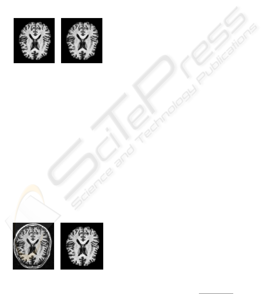
Figure 2 illustrates the effect of the anisotropic
diffusion filter on MRI brain. In our case, the param-
eter time step was 0.125, the number of iterations was
5, and the conductance value was 3.0. In This result
we show how the volume data is smoothed and edges
are preserved.
Figure 2: Effect of the anisotropic diffusion filter on an MRI
brain image. (left) original data, (right) smoothed data.
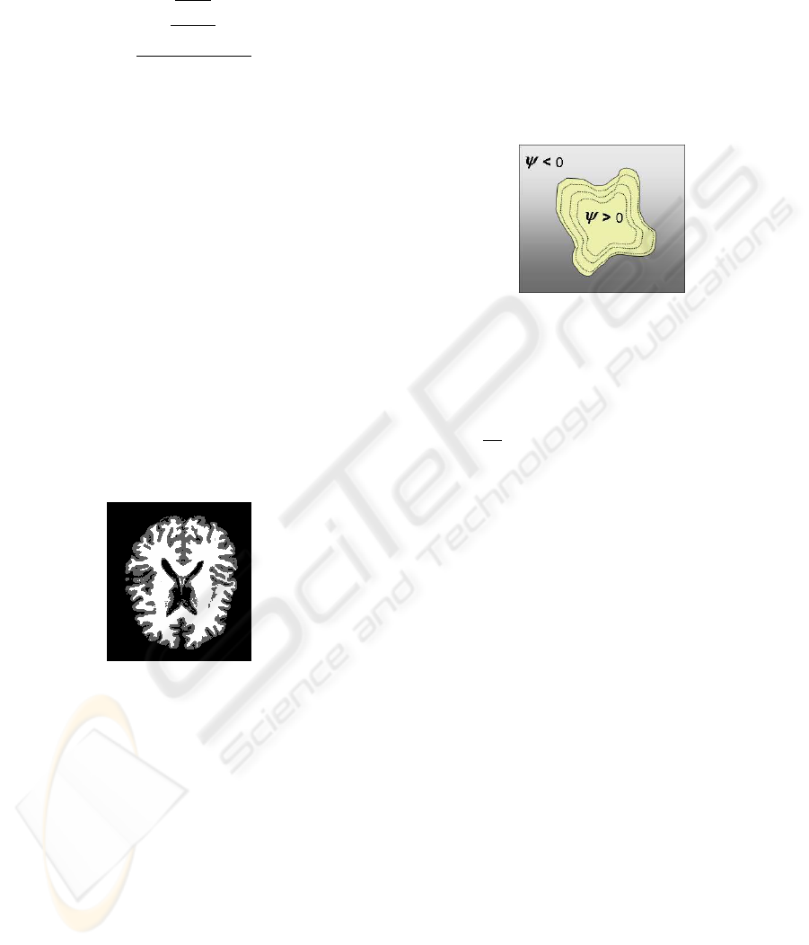
2.2 Non-Brain Tissue Removal
Removal of non brain tissue from the MR volume
can facilitates later stages in the algorithm as fewer
voxels and fewer tissue types are involved. On the
other hand, only brain tissue is retained and all non-
brain tissues are masked out. A number of techniques
have been proposed for brain mask extraction from
MRI data. Here, we have applied the standard tech-
nique called -Brain Extraction Tool (BET)- which has
been proposed by Smith et al. (Smith, 2002). This
algorithm uses deformable model technique, which
evolves to fit the brain’s surface by the application of
a set of locally adaptive model forces. It can remove
skull, scalp, and other tissue from the MR image. An
illustration of this process is shown in figure 3.
Figure 3: Removal of extracerebral tissues. (left) original
image, (right) cerebral structures.
2.3 Downsampling Volume
In computer graphics, downsampling (or ”resam-
pling”) is the process of reducing an image to a
smaller size. Changing the pixel dimensions of an
image is called also resampling. The downsampling
process is an important task in image analysis that
decreases computation time and improves rendering
performance. Therefore, an improvement in speed
could be gained by downsampling the initial volu-
metric data before any other processing. The gain in
speed could be obtained by the reduction of the num-
ber of voxels. For example if the dimension of an
input MRI volume is 256 x 256 x 150 voxels and if
this MRI was downsampled from 1.0 mm
3
to (2.0 x
2.0 x 5) mm
3
in the x-, y- and z-directions respec-
tively, then the output volume dimensions are 128 x
128 x 30 voxels. Therefore, downsampling the input
volume of 9,830,400 voxels to an output volume of
491,520 voxels drops out 95% of the voxels from the
input volume. Thus, next statistical estimation will be
performed by the resampled data and level-set evolu-
tion will be done on original smoothed volume.
2.4 Estimation Maximization
The classification step is intended to provide an initial
model that can be refined using level-set. In the case
of unsupervised classification, the Expectation Max-
imization (EM) algorithm (Dempster et al., 1977), is
an efficient iterative procedure to compute the Max-
imum Likelihood (ML) estimate in the presence of
hidden data f. In short, the EM algorithm alternates
between two steps: an expectation (E) step and a max-
imization (M) step. In the E-step, the missing data
are estimated given the observed data and current esti-
mate of the model parameters. In the M-step, we com-
pute the maximum likelihood estimates of the param-
eters by maximizing the expected likelihood found in
the E-step. The parameters found in the M-step are
then used to begin another E-step, and the process
is repeated. The method classifies resampled image
into white matter (WM), grey matter (GM) and cere-
brospinal fluid (CSF).
Let us consider the mean parameter µ
k
and the
variance parameter σ
k
of the intensity distribution
of the k-th tissue class grouped in θ
k
such as θ
k
=
{µ
k
,σ
k
}. We denote also π
k
the prior probability of
each class k and γ
k
i
the posteriori probability calcu-
lated in each voxel i for each class k. In the expec-
tation step, we calculate the posteriori probability ac-
cording to the following formulas:
γ
k
i
= P(x
k
/y
k
,θ
k
) =
π
k
i
f
k
(y
i
/θ
k
)
∑
K
l=1
π
l
i
f
l
(y
i
/θ
l
)
(2)
A FAST AND ROBUST METHOD FOR VOLUMETRIC MRI BRAIN EXTRACTION
463
In the maximization step, we estimate data driven
parameters by:
π
k
=
∑
K
l=1
γ
k
i
N
µ
k
=
∑
K
l=1
γ
k
i
y
i
∑
K
l=1
γ
k
i
σ
2
k
=
∑
K
l=1
γ
k
i
(y
i
−µ
k
)(y
i
−µ
k
)
∑
K
l=1
γ
k
i
(3)
2.5 Clustering
Gaussian parameters obtained previously on the
downsampled volume are generally identical to those
obtained on whole volume. In this way, an improve-
ment in speed could be gained in the clustering step.
At this step, classification is restricted to three classes:
gray matter (GM), white matter (WM) and CSF. Sev-
eral classifiers could do this task such as k-means,
Fuzzy k-means, k-NN, etc. However, we show that
a simple clustering based on euclidian distance is suf-
ficient. More precisely, each voxel is assigned to one
class based on its minimum euclidian distance. This
simple way decreases also computation time and pro-
vides good results. Figure 4 illustrates the effect of
this clustering with three classes. The mean values
are estimated by the EM algorithm.
Figure 4: Clustering of the MR image (original image is
shown in figure 3).
2.6 Level-set Method
The aim of this step is to extract accurately the bound-
ary of the region-of-interest by using a deformable
level-set model. Therefore, we exploit previous ini-
tialization to accelerate and to guide the process evo-
lution. Level set method, initially introduced by Os-
her and Sethian (Osher and Sethian, 1988), has been
used in many applications: physics, graphics, com-
puter vision, image analysis, restoration, etc. It be-
comes also one of the popular frameworks for image
segmentation. Theoretically, the level set function ψ
will change with time according to the speed term F
(as illustrated in the eq. 6) and the front Γ is always
represented by the zero isosurface. ψ and Γ are de-
fined as follows:
ψ :
Ω × [0,+∞[→ IR
(x,y,t) 7→ ψ(x,y,t)
ψ(x,y,t = 0) = ±d(x, Γ)
(4)
Γ(t) = {(x,y) ∈ Ω;ψ(x, y,t) = 0} (5)
Figure 5: Level-set concept.
ψ(t) takes opposite signs on each side of Γ(t) (Fig.5).
The evolution of ψ(t) can be expressed as:
∂ψ
∂t
= F|∇ψ| = αP(x)|∇ψ| + βk|∇ψ| (6)
Where P(x) is a propagation (speed) term that con-
trols surface expansion/contraction and k is a curva-
ture term that controls the smoothness of the surface.
α and β are scalar constants. The standard convention
for level-set segmentation is that positive propagation
term causes the surface to expand while negative term
causes the surface to contract.
Different implementations of the level-set func-
tion are proposed in literature (Sethian, 1996). We no-
tice that most of them are relatively sensitive to initial
conditions. For best efficiency, the initial front should
be the best guess possible for the solution. Here, we
expect two inputs for our implementation. The first is
an initial front, which is given by previous step (i.e.
statistical classification), and the second is a feature
image from which the propagation term P(x) is cal-
culated (see eq. 4). In the feature image, values that
are close to zero are associated with object bound-
aries and speed term is calculated as the laplacian of
the image. The goal is to attract the evolving level set
surface to local zero-crossings in the laplacian image.
One nice property of using the laplacian is that there
are no free parameters in the calculation and it is of-
ten used for edge detection. Finally, positive values
in the output image are inside the segmented region
and negative values are outside. The zero crossings of
the image correspond to the position of the level set
front.
VISAPP 2008 - International Conference on Computer Vision Theory and Applications
464
2.7 3D Volume Rendering
Representing the surface as an explicit geometry is
efficient when used with the conventional computer
graphics approaches for shading and viewing. Fur-
ther, it greatly reduces the necessary data storage and
provides a data structure that can be measured. At
this step, our segmentation is transformed into a tri-
angulation using an isosurface ”marching cubes” al-
gorithm (Lorensen and Cline, 1987). More precisely,
an isosurface is a surface that passes through all lo-
cations in space where a continuous data volume is
equal to a constant value. However, the output trian-
gulated surfaces usually contains multiple small ”use-
less” meshes that are physically disconnected from
each other. In order to reduce aliasing artefacts and
produce a smooth surface estimation, we have ap-
plied the algorithm proposed by Whitaker (Whitaker,
2000).
3 EXPERIMENTAL RESULTS
At this stage, we have validated the performance of
the proposed method on some 3D MRI data sets.
Clustering process is limited to provide only three
classes: GM, WM and CSF because our first objective
is to prove speed and not to extract all internal tissues.
In the first experiment, two different axial MRI data
sets consisting of 181 slices have been tested. The
voxel size is 1 mm
3
. Figure 7 shows the final seg-
mented white matter tissue.
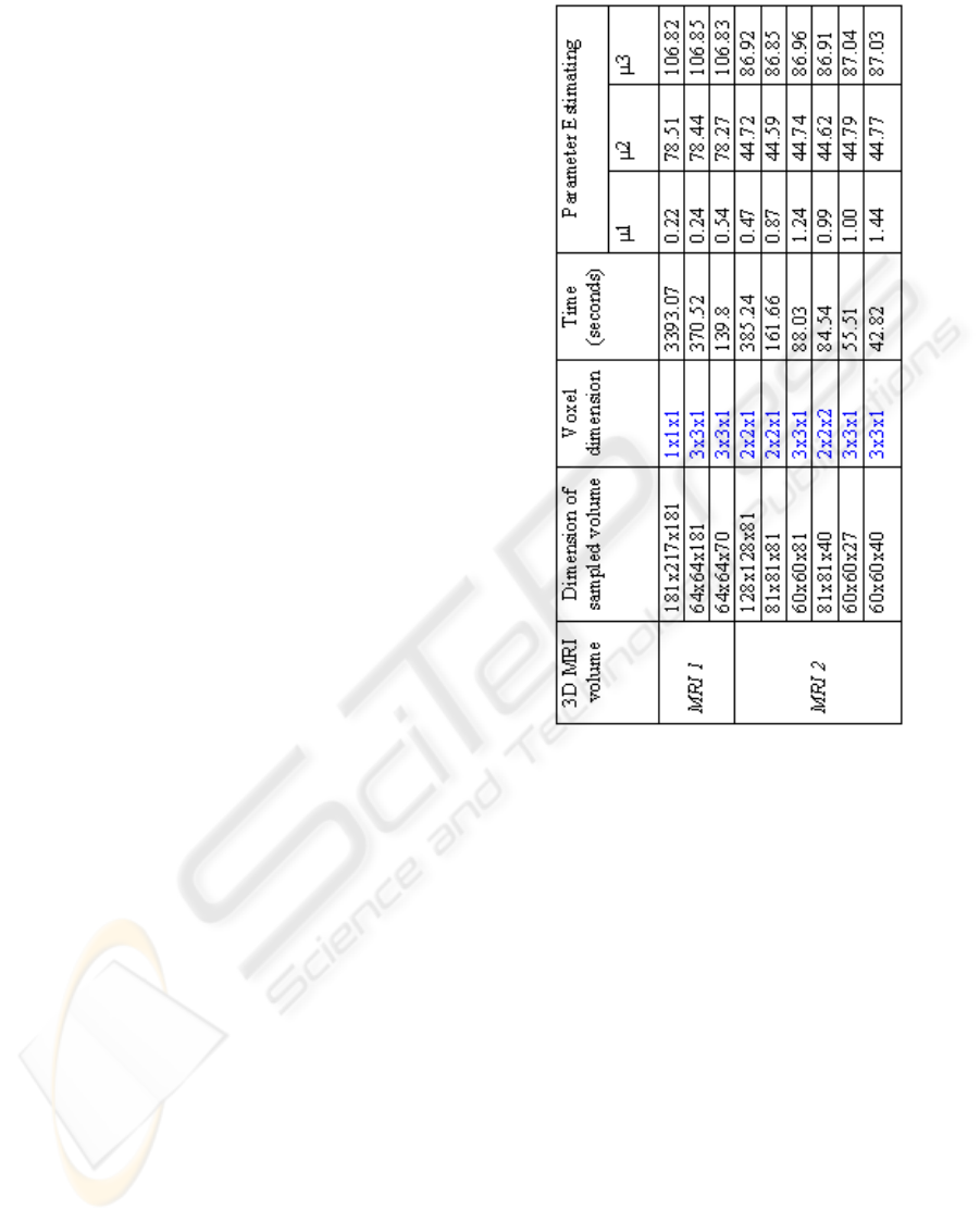
Figure 6 shows the cpu time and the gaussian pa-
rameters obtained by our method. Processing was
performed on a 1.5 Mhz Intel Pentium HP with 512
MB of RAM. The second column of the table presents
different sample sizes of two initial data sets. The
fourth column is reserved for the computation time.
The three last columns illustrate mean values of the
three classes (CSF, GM, WM) which are estimated by
EM. According to these results, we notice that mean
values of each class are almost the same ones to all
samples and a notable gain in computation time was
performed. However, the current process can provide
poorer quality. For example, when we resample an
image to larger pixel dimensions, the image will lose
some detail and sharpness.
For instance, these first results are encouraging but
further investigation is required to extend the algo-
rithm to a large range of data.
Figure 6: CPU times (in seconds) and parameter estimation
provided by our algorithm : application on two normal MR
Data with different samples.
4 CONCLUSIONS
In this paper, we have proposed method for 3D MRI
brain segmentation problem. We have explored the
use of deformable level-set models to segment ac-
curately different brain tissues. The algorithm gives
satisfying results for brain tissues segmentation. It is
also relatively computationally efficient and fast. At
this stage, we have only presented preliminary results
to demonstrate its potential: Even if they have not yet
been compared to manual or other automatic segmen-
tation results, we think that they are encouraging and
faster than manual procedures.
However, clinical validation remains to be done,
which will require additional work. Future valida-
tions will compare our segmentation with manually
labelled data and other segmentation results. Future
work could be the integration of anatomical knowl-
A FAST AND ROBUST METHOD FOR VOLUMETRIC MRI BRAIN EXTRACTION
465
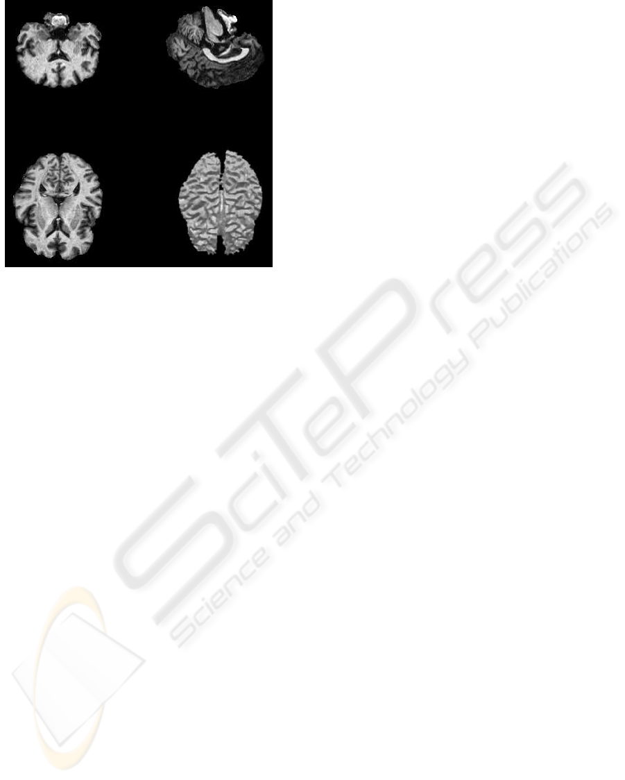
Figure 7: White matter segmented using our implementa-
tion.
edge to improve segmentation performance. Finally,
the same framework can be used and extended to seg-
ment and quantify abnormal brains.
REFERENCES
Davatzikos, C. and Bryan, R. (1996). Using a deformable
surface model to obtain a shape representation of the
cortex. IEEE Trans. Med. Imag, 15:785–795.
Dempster, A., Laird, N., and Rubin, D. (1977). Maximum
likelihood from in complete data via the em algorithm.
Journal of the Royal Statistical Society, 1:1–38.
Kass, M., Witkin, A., and Terzopoulos, D. (1987). Snakes:
Active contour models. Int. J. Comput. Vis., 1:321–
331.
Lorensen, W. and Cline, H. (1987). Marching cubes:
A high-resolution 3-d surface construction algorithm.
ACM Comput. Graph, 21:163–170.
Osher, S. and Sethian, J. (1988). Fronts propagating
with curvature-dependent speed: Algorithms based on
Hamilton-Jacobi formulations. Journal of Computa-
tional Physics, 79:12–49.
Perona, P. and Malik, J. (1990). Ieee transactions on pat-
tern analysis machine intelligence. IEEE Trans. Med.
Imaging, 12:629–639.
Pham, D., Xu, C., and Prince, J. (1998). A survey of current
methods in medical image segmentation. Technical
report, Johns Hopkins University, Baltimore.
Sandor, S. and Leahy, R. (1997). Surface-based labeling
of cortical anatomy using a deformable atlas. IEEE
Trans. Med. Imaging, 16:41–54.
Sarang, L. (2000). 3D segmentation techniques for medical
volumes. Technical report, State University of New
York at Stony Brook.
Sethian, J. (1996). Level set methods and fast marching
methods. Cambridge University Press.
Shattuck, D., Leahy, S. S., Schaper, K., Rottenberg, D., and
Leahy, R. (2001). Magnetic resonance image tissue
classification using a partial volume model. Neuroim-
age, 13:856–876.
Smith, S. (2002). Robust automated brain extraction. Hu-
man Brain Mapping, 17:143–155.
Suri, J., Singh, S., and Reden, L. (2002). Computer vision
and pattern recognition techniques for 2-d and 3-d mr
cerebral cortical segmentation (part i): A state-of-the-
art review. Pattern Analysis and Applications, 5:46–
76.
Whitaker, R. (2000). Reducing aliasing artifacts in iso-
surfaces of binary volumes. IEEE Volume Visualiza-
tion and Graphics Symposium, 21:23–32.
Xu, C., Pham, D., Rettmann, M., Yu, D., and Prince, J.
(1999). Reconstruction of the human cerebral cortex
from magnetic resonance images. IEEE Transactions
on Medical Imaging, 18:467–480.
VISAPP 2008 - International Conference on Computer Vision Theory and Applications
466
