A SLAG TEMPERATURE AND FLOW MONITORING SYSTEM

Jean-Philippe Andreu

Joanneum Research, Institute of Digital Image Processing, Wastiangasse 6, A-8010 Graz, Austria

Keywords: Optical high temperature measurements, slag monitoring, industrial vision, motion tracking, optical flow.

Abstract: Quality assessment of steel processing essentially relies on the continuous monitoring and control of the

steel temperature and the flow patterns of the molten material. Among the various sensors developed to

control that process, CCD cameras emerge as a good alternative to more classical measuring devices. Multi-

spectral imaging systems based on cameras working in the visible spectrum offer a viable alternative to high

cost thermographic infrared cameras. This paper presents a slag monitoring system based on dual

wavelength thermographic cameras. The system allows a real-time and contactless monitoring of the slag

temperature and a continuous monitoring of the flow patterns of the ingot slag topping in order to assess the

quality of the produced steel.

1 INTRODUCTION

Precisely controlling the solidification of liquid steel

is one of the cornerstones in quality steel making.

By varying the amount of heating, usually by

adjusting the current going through an electrode

immersed the liquid steel one can precisely control

the solidification process. This is why monitoring

the temperature of the liquid phase of the steel is of

great importance to steel producers.

Given the very high temperatures of liquid steel

and the slag on top of it (usually between 1300°C

and 1800°C) and the particularly harsh environment

at the producing plant, only very few sensors

(usually thermocouple probes and pyrometers) are

able to accurately measure the temperature of the

steel. Conventionally, for measuring the temperature

an operator has to immerse a probe with a

thermocouple into the liquid steel slag at periodic

intervals. Since thermocouple probes cannot work

reliably under the influence of the high currents, the

heating electrode has to be removed from the mould

before a measurement is done. This periodic

removal of heating power disturbs the solidification

process. An alternative way of measuring the

temperature was therefore sought, provided that it

can guarantee at least the same accuracy as

thermocouple probes: +/- 5 °C.

Due to their high cost thermographic infrared

cameras were often discarded as an option. At a

fraction of the cost of infrared cameras a dual

wavelength camera solution working in the visible

spectrum offers a viable alternative (Meriaudeau,

2003). Such a system can deliver images of high

spatial resolution while at the same time measuring

temperature with an accuracy better than +/- 5 °C.

Using thermal cameras is also beneficial to the

observation of the flow patterns of the molten

material. That important process information was

until now only estimated by a trained operator.

Still it is pretty hard to determine the

temperature of liquid steel from images. Within an

image of the surface one can see regions where the

material forms a “crust” (i.e. “cold” regions), while

other regions display a laminar flow of hot material

from below up to the surface with from time to time

spontaneous “bubbles” bringing up hot liquid at a

fast rate. One of the difficult tasks for an image

processing algorithm is therefore to distinguish those

areas and at the same time yield a accurate

temperature.

2 TEMPERATURE MEASURE

2.1 Monochromatic Method

Contactless temperature measurement is based on

the analysis of the radiations emitted by the object

under inspection. Planck’s law relates the

502

Andreu J. (2008).

A SLAG TEMPERATURE AND FLOW MONITORING SYSTEM.

In Proceedings of the Third International Conference on Computer Vision Theory and Applications, pages 502-507

DOI: 10.5220/0001074305020507

 SciTePress

electromagnetic energy radiated from a black body

to its absolute temperature:

()

1exp

−

⎟

⎠

⎞

⎜

⎝

⎛

⋅=

πλ

(1)

with

the temperature,

the wavelength,

πλ

the

first radiation constant: 1.191062

×10

Wμm

-1

, C

the second radiation constant: 1.438786

×10

Wμm

and

the spectral radiance. As ideal emitter a

black body emits the maximum radiation compared

to any other object for a given temperature. The non-

ideal behaviour of real objects is generally

accounted by the emissivity

. It corresponds, for

the same spectral wavelength

, to the ratio of the

actually emitted total radiation to its theoretical

maximum (i.e. black body radiation). Since

≤

the apparent temperature of a real object measured

by a radiometer is always lower than its true

temperature. A derivation of Eq. (1) is then used to

determine the true target temperature

from the

measured temperature

λλ

CTT

(2)

Due to surface properties and experimental

conditions determining a reliable value for

can

prove a difficult and error prone task.

2.2 Dual-wavelength Method

Measuring temperature with a dual wavelength

method was first introduced by Campbell et al.

(Campbell, 1925). The method consists in measuring

the ratio of two spectral radiances. Using spectral

filters, two radiances emitted by the object are

acquired simultaneously at two different

wavelengths

and

. The temperature

λλ

then inferred from the ratio temperature

λλ

CTT

λλλλ

2,,

2121

(3)

being the ratio wavelength:

λλ

−

(4)

being the ratio emissivity:

(5)

And

⎟

⎠

⎞

⎜

⎝

⎛

−

TTT

2121

21,

λλλλ

λλ

(6)

According to Eq. (3), the ratio temperature

λλ

corresponds to the true target temperature

λλ

whenever

and

are equal (i.e.

)

which is the definition of a gray body.

2.3 System Layout

Urban et al. (Urban, 2005), following Meriaudeau et

al. (Meriaudeau, 2003), presented a temperature

measurement system composed of a beam splitter

and two CCD cameras equipped with different

interferential filters. That system, based on dual

wavelength, estimates the temperature of gray

bodies with a maximum error of 0.5% of the

experimental temperature range with the assumption

that the emissivity does not change too much as a

function of the wavelength (i.e. gray body

assumption). In other words,

and

have to be

chosen sufficiently close from each other while at

the same time distant enough to allow sufficient

sensitivity of the instrument.

That system has several advantages. As long as

the gray body assumption holds the measured object

and the calibration object do not need to be of the

same material. This means the measuring instrument

can be calibrated with one radiation source (e.g. a

tungsten filament inside a lamp bulb) but can then be

used to measure the temperature of another object of

totally different material (e.g. the molten slag).

Another advantage of the dual wavelength approach

is its inherent robustness with regard to dust. Dust

depositing on the front lens will equally influence

intensities measured at both wavelengths and

therefore does not deteriorate the measurement

accuracy.

2.4 Practical Considerations

Under immediate vicinity to the melting process the

system must still reliably perform under

environmental challenges such as:

 Extreme heat radiation from the melted steel:

The camera system is built into a massive

housing, an extra air cooled radiation shield is

needed to keep the cameras within their specified

operating temperature range (i.e. below 50°C).

 Extremely strong magnetic fields in the vicinity

of the melting electrode: Proper choice of

location and heavy magnetic shielding of the

A SLAG TEMPERATURE AND FLOW MONITORING SYSTEM

503

camera housing and the cabling have to be taken

into account.

 High levels of dust / smoke during the process:

All the sensitive optics and electronics have been

built into a fully sealed housing while a circular

ventilation slit around the first optical element in

the system (heat protection filter) avoids

deposition of dust.

 Gears occluding the camera field of view: The

gear manipulating the heating electrode can

temporarily occlude the camera field of view

therefore the measurement location has to be

chosen with care.

Because calibrated blackbodies were only

available up to 1500°C and the temperatures under

consideration are above the fusion point for most

metals an alternative approach was chosen to

calibrate the instrument up to 2000°C. The

relationship between the temperature and the current

of a 250 W halogen lamp was established using a

classic Hartmann und Braun filament pyrometer.

The tungsten filament of the halogen bulb was used

as a rough calibration. For better accuracy a NIST

traceable black body can be used for calibration.

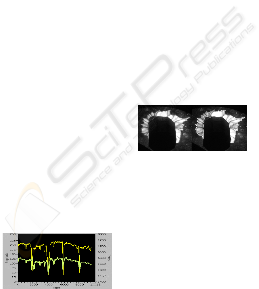
2.5 Temperature Measurement Results

Temperature measurement results are shown in

Figure 1. The curves represent about 2.5 hours of the

process at a sampling rate of one measurement per

second. The deep notches in the temperature curves

show the influence of a thermocouple measurement:

when the electrode is taken out, the fluid steel

circulation stops resulting in a sharp drop in surface

temperature. The upper curve represents the

measurement of the hottest spot (typically a bubble

rising from below the slag surface). The lower curve

displays the average temperature over the whole

liquid steel surface. That curve correlates quite well

with thermocouple measurements. The most precise

measurements come from measuring the temperature

from areas that are reliably visible at all stages of the

process such as large laminar flowing areas that

bring up to the surface a continuous stream of hot

material.

Figure 1: Temperature measurement results.

3 FLOW MONITORING

During the steel producing process the flow pattern

of the slag is a visible indicator of the process

quality. Currently a worker checks on an irregular

basis the slag motion and interprets its motion. In a

qualitative manner the motion can be specified as

‘good’ if the direction of the homogeneous slag is

flowing towards the electrode from all directions.

On the other hand if the slag flows from the centre

of the electrode towards the border of the mould the

slag motion is qualified as ‘bad’.

3.1 Active Slag Region of Interest

To speed up the qualitative slag motion computation

we restrict ourselves to the most active regions

where the most active motion will be observed.

Contrary to regions where the slag is solidified

(i.e. cold slag), active regions are the hottest and

therefore correspond to the regions with the highest

intensity in the images of the slag. Segmenting these

regions is simply performed by an optimal

thresholding method (Otsu, 1979) and by discarding

the regions of too small area. Figure 2 shows the

segmentation result on a test image.

Figure 2: Segmented image region of slag active motion.

3.2 Slag Motion Analysis

In an image sequence the moving patterns of the slag

cause temporal variations of the image brightness. If

we assume that all temporal intensity changes are

due to motion only, analysing the slag motion

requires to compute how much each image pixel

moves between adjacent images. For determining

the motion parameters we use a pyramidal variant

(Bouguet, 2000) of the well-known tracking

algorithm presented by Lucas and Kanade (Lucas,

1981). This algorithm was chosen because it is

general enough, reliable, robust and fast enough to

handle the required frame rate of our monitoring

system.

VISAPP 2008 - International Conference on Computer Vision Theory and Applications

504

3.2.1 Motion Tracking

The basis of the Motion Constraint Equation

assumes that if

),( yxI

is the centre pixel of

neighbourhood

Ω and moves by a displacement

vector

()

yxd

within an adjacent image J

(with

)( tIJ

), since

),( yxI

and

),( yyxxJ

represent the same point one

can write:

),,(),,( ttyyxxItyxI

(7)

Providing that

and

are not too big, one

can perform a first order Taylor series expansion

about

),,( tyxI :

εδδδ

∂

+= t

tyxI ),,()7(

(8)

where

is assumed to be small and can be

neglected. Using Eq. (7) and Eq. (8) we obtain:

0=++

tyyxx

(9)

Where

and

are the components

of the image velocity and

∂

and

∂

are the image intensity derivatives. Eq. (9)

can be rewritten more compactly as:

−=⋅∇

(10)

where

),(

=∇

is the spatial intensity

gradient and

),(

is the image velocity or

optical flow at pixel

)

(

at time t.

A weighted least-squares fit of the local first-

order constraints of Eq. (10) to a constant model for

in each small spatial neighbourhood Ω can be

implemented by minimizing:

[

]

∑

Ω∈

+⋅∇

tyxItyxIyxW

),,(),,(),(

(11)

where

)

(

denotes a window function that

gives more influence to constraints at the centre of

the neighbourhood than those at the periphery.

)

(

are typically 2D Gaussian coefficients but

can be set to 1.0 with little effect on the accuracy.

The solution to Eq. (11) is given by:

[

]

bAAA

−

(12)

where for

N pixels in

at a single time t:

[

]

),(),...,,(

11 NN

∇

(13)

(

)

),(),...,,(

11 NNtt

yxIyxIb

−

(14)

The solution to Eq. (12) can be solved in closed

form when

is a non-singular matrix:

⎥

⎦

⎤

⎢

⎣

⎡

∑∑

∑

Ω∈Ω∈

yxIyxIyxI

),(),(),(

(15)

3.2.2 Accuracy and Robustness

The two key components for determining the optical

flow are accuracy and robustness. The accuracy

component relates to the ability of taking into

account the details contained in the images.

Intuitively, a small neighbourhood

would be

preferable in order not to “smooth out" image

details. The robustness component relates to the

sensitivity to changes of lighting, size of image

motion, etc... In particular, in order to handle large

motions, it is intuitively preferable to pick a large

neighbourhood

. Therefore there is a natural

trade-off between local accuracy and robustness

when choosing the neighbourhood size.

In order to provide a solution to that problem,

we use a pyramidal implementation of the classical

Lucas-Kanade algorithm (Bouguet, 2000). In that

variant implementation an image pyramid is first

built by recursively sub-sampling (by a factor of 2)

the highest resolution image up to a user defined

pyramid height/level

. The optical flow is

computed at the deepest pyramid level

and

propagated to the upper levels up to level 0 (the

original image). The final solution

is the sum of

the residual pixel displacement vectors available

after the finest optical flow computation:

∑

. The clear advantage of a pyramidal

implementation is that it allows large pixel

displacements, while keeping the size of the

neighbourhood relatively small.

3.2.3 Differentiation

Image intensity derivatives are required for

computing the optical flow. Differentiation is done

using matched balanced filters (Simoncelli, 1994) of

A SLAG TEMPERATURE AND FLOW MONITORING SYSTEM

505

size 5 for low pass filtering (e.g. blurring) and high

pass filtering (e.g. differentiation). Matched filters

allow comparisons between the signal and its

derivatives as the high pass filter is simply the

derivative of the low pass filter and, from

experimental observations, yields more accurate

derivative values.

For instance for computing

, we first

convolve with the low pass filter in the

t dimension

to reduce 5 images to one, then convolve that image

with the same filter in the

y dimension and finally

convolve with the differentiation filter in the

dimension to obtain

3.2.4 Tracking Points

Instead of tracking all the points within areas where

the slag is active, we limit ourselves to tracking

featured points. Following Shi and Tomasi (Shi,

1994) the selection of featured points is more than a

traditional measure of “interest”: it is determining

the right features that make the tracker work best.

A measure of “textureness” is derived over

non-overlapping square windows of size 15 in the

areas of interest. That measure is based on the

assumption that if the inter-frame displacement is

sufficiently small with respect to the texture

fluctuations within the window, the displacement

vector can be found minimizing the error residue:

(

)

[

]

dxwxJdxI

∫

−−=

)(

(16)

In this expression,

w is a weighting function

and could be set to 1 or alternatively, could be a

Gaussian-like function that emphasizes the central

area of the window. Solving that linear system

requires the coefficients to be both above the image

noise level and well conditioned. Using Singular

Value Decomposition (SVD) for solving the system

and one can decide by examining the resulting eigen

values (e.g. the smallest of the eigen values should

be superior to a user specified threshold) if the

system well conditioned and if the window is a valid

one for that measure.

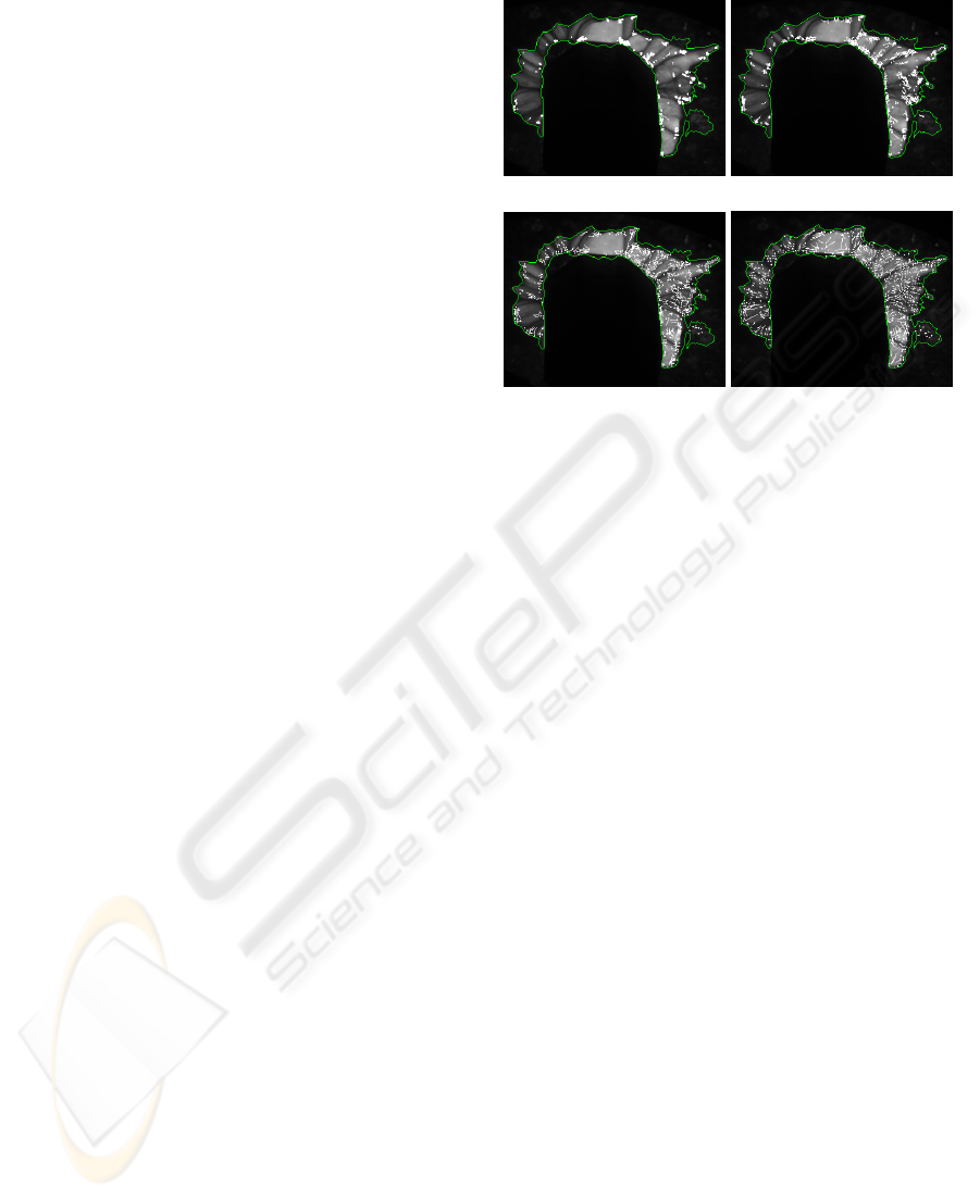
In order to avoid tracking too many feature

points we restrict their number to a user defined

value (e.g. from 600 to 1000). To prevent the feature

points to be crowded in some few spots, which

results in a poor distribution of trackable points (see

Figure 3), we use a parameter to specify the desired

minimum distance (in pixels) between the candidate

points. Experience showed that using a minimum

distance of 4 pixels delivers good results in well

distributing the points. Increasing this factor too

much results in poor tracking resolution because the

points get spread too far apart.

Minimum distance = 0 Minimum distance = 2

Minimum distance = 3 Minimum distance = 4

Figure 3: Effect of different minimum distance values on

tracking point distribution.

3.2.5 Re-initialisation of Tracking Points

During the tracking process the algorithm tries to

track every feature point found at the initialization

step over the next frames. If the point is lost for

instance by moving out of the active slag area or by

not being identified again in the new frame, the

algorithm initializes (using the procedure described

in the previous section) a new point for the one lost

to keep the total number of tracking points constant.

3.3 Finding the Electrode Centre

Before analyzing the overall slag motion we first

have to define a reference point, which the motion of

the slag can be related to. We use the approximate

centre of the electrode as reference point.

Starting from the resulting image mask by

segmenting the region of active slag motion (Figure

4 left), this mask contour is first converted into a

polygon. From this polygonal representation the

convex hull is computed.

The convex hull of a set of points is the

intersection of all convex sets containing that set.

For N points

,...,

the convex hull is then given

by the expression:

⎭

⎬

⎫

⎩

⎨

⎧

=∀≥≡

∑∑

andjpC

1,0:

λλλ

(17)

From the convex hull the centre of mass (Figure

4 right) is computed and taken as an approximation

for the centre of the electrode which is used to relate

VISAPP 2008 - International Conference on Computer Vision Theory and Applications

506

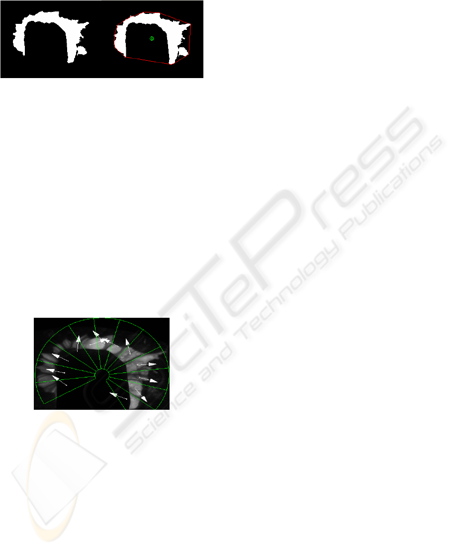
the direction of the tracking vectors for analysing the

slag motion.

Figure 4: The electrode centre as the convex hull centroid.

3.4 Direction of the Slag Flow

To determine the overall slag motion, the region of

active slag motion is divided into sectors of a circle

centred at the approximated electrode centre (Figure

5). The number of sectors and the distance between

them is user dependant. Experiments showed that in

combination with 600 to 1000 tracking points, 12

sectors delivered good results.

Within each sector the tracking vectors are

accumulated into a histogram of directions. To

improve robustness in detecting the main direction

in each sector we do not take into account vectors

whose length do not exceed 3 pixels. Finding the

maximum in the directional histogram provides the

preferred direction of the slag motion of the

considered sector. Figure 5 displays the main

directions found for each sector.

Figure 5: Sectors of active slag areas and detected flow.

For the final quantification of the slag motion,

we have to determine if most of the slag is moving

towards the electrode or in the opposite direction.

For this purpose each vector direction is compared

to the direction of the sector they belong to. The

direction of a sector is simply the direction of the

line bisecting the sector towards the centre of the

electrode. If the absolute angular difference between

a vector direction and the direction of its sector lays

within a range of 0-60° the slag motion for this

vector is “good”, if the absolute difference is

between 60° and 120° the slag motion is

“undetermined” and otherwise the slag motion is

“bad”. For quantifying the overall slag motion in a

given sector a majority voting is performed among

the slag motion vectors belonging to the same sector.

4 CONCLUSIONS

We presented an experimental industrial vision

system capable of measuring the slag temperature in

a contactless manner with an accuracy of ± 5° C. By

tracking the flow patterns of the slag, that system

can also monitor and help assessing the quality of

the produced steel. As future development we plan

on investigating the relationship between the slag

motion flow and its temperature in order to give the

operator a better insight about the produced steel.

ACKNOWLEDGEMENTS

This work has been carried out within the K plus

Competence Centre Advanced Computer Vision.

This work was funded from the K plus Program.

REFERENCES

Bouguet, J.-Y. (2000) ‘Pyramidal Implementation of the

Lucas Kanade Feature Tracker: Description of the

Algorithm’, OpenCV Documents, Intel Corporation,

Microprocessor Research Labs.

Campbell, N. R.; Gardiner, H. W. B. (1925) ‘Photo-

electric colour-matching’, Journal of Scientific

Instruments, Vol. 2, Issue 6, pp. 177-187.

Lucas, B.D.; Kanade, T. (1981) ‘An Iterative Image

Registration Technique with an Application to Stereo

Vision’, Proceedings of the 7th International Joint

Conference on Artificial Intelligence, pp. 674-679.

Meriaudeau, F.; Legrand, A.C.; Gorria, P. (2003) ‘Real-

time multispectral high-temperature measurement:

application to control in the industry’, Proceedings of

the SPIE, Vol. 5011, pp. 234-242.

Otsu, N. (1979); ‘A threshold selection method from gray-

level histograms’, IEEE Transactions on Systems,

Man and Cybernetics, Vol. 9, pp. 62-66.

Urban, H.; Sidla, O. (2005); ‘Online Temperature

Measurement and Flow Analysis of Hot Dross in a

Steel Plant’, Proceedings of the SPIE, Vol. 6000, pp.

66-74.

Shi, J.; Tomasi C. (1994); ‘Good Features to Track’,

Proceedings of the IEEE Conference on Computer

Vision and Pattern Recognition, Vol. 1, pp593-600.

Simoncelli, E.P. (1994); ‘Design of multi-dimensional

derivative filters’, Proceedings of the IEEE Int.

Conference on Image Processing, Vol. 1, pp790-793.

A SLAG TEMPERATURE AND FLOW MONITORING SYSTEM

507