
ACCURACY IMPROVEMENTS AND ARTIFACTS REMOVAL IN
EDGE BASED IMAGE INTERPOLATION
Nicola Asuni
Dipartimento di Informatica, Universit`a degli Studi di Cagliari, via Ospedale 72, Cagliari, Italy
Andrea Giachetti
Dipartimento di Informatica, Universit`a degli Studi di Verona, Strada Le Grazie, 15, Verona, Italy
Keywords:
Interpolation, Edges, Artifacts, Image quality.
Abstract:
In this paper we analyse the problem of general purpose image upscaling that preserves edge features and
natural appearance and we present the results of subjective and objective evaluation of images interpolated
using different algorithms. In particular, we consider the well-known NEDI (New Edge Directed Interpolation,
Li and Orchard, 2001) method, showing that by modifying it in order to reduce numerical instability and
making the region used to estimate the low resolution covariance adaptive, it is possible to obtain relevant
improvements in the interpolation quality. The implementation of the new algorithm (iNEDI, improved New
Edge Directed Interpolation), even if computationally heavy (as the Li and Orchard’s method), obtained, in
both subjective and objective tests, quality scores that are notably higher than those obtained with NEDI and
other methods presented in the literature.
1 INTRODUCTION
Image upscaling through pixel interpolation is used in
different fields to create high resolution images with
a ”natural” appearance from low resolution acquired
data. Applications of this procedure can be found
in image viewing/processing software, photographic
printing and Computer Graphics. Real time algo-
rithms can also be applied to increase the perceived
quality of video streaming or textures in virtual navi-
gation tools.
In general, the procedure tries to recover missing in-
formation by assuming that there is a known relation-
ship between a low resolution image and the same im-
age acquired with an high resolution sensor. General
purpose algorithms for the upsampling of single im-
ages, unlike methods that use multiple images to gen-
erate high resolution ones (usually referred as super-
resolution algorithms) do not add real information on
the scene and are not useful as pre-processing steps
in vision based applications. They are, however, in-
teresting for researcher due to the necessity of remov-
ing pixelization, blurring and other annoying artifacts
affecting images enlarged with trivial techniques (i.e
pixel replication or bilinear interpolation). Several al-
gorithms have been therefore proposed in literature to
obtain better results and several patents have been ob-
tained for ”smart” interpolation techniques.
Few systematic comparisonshavebeen, however, pre-
sented and it is difficult to determine which method is
the best suited for a selected application. In this paper
we present (section 2) a short review on the methods
proposed for image upsampling. We then focus our
attention on the NEDI method (Li and Orchard, 2001)
that seem to provide very good results, even if at the
cost of a large computational complexity that limits
its fields of application. We analyse (section 3) the
drawbacks of the method and propose a modified al-
gorithm (iNEDI, improved New Edge Directed Inter-
polation) that reduces the effects of most of them. In
section 5 we show that the new method provides the
best results in a large set of objective and subjective
tests performed to compare the quality of differently
upsampled natural images.
2 INTERPOLATION
APPROACHES: A REVIEW
The simplest image interpolation algorithms are
based on linear filtering. Values of the new pixels
are obtained by assuming that the values of the image
58
Asuni N. and Giachetti A. (2008).
ACCURACY IMPROVEMENTS AND ARTIFACTS REMOVAL IN EDGE BASED IMAGE INTERPOLATION.
In Proceedings of the Third International Conference on Computer Vision Theory and Applications, pages 58-65
DOI: 10.5220/0001074100580065
Copyright
c
SciTePress
function in the new pixel locations can be computed
as a linear combination of the values of the original
pixels close to the new position. Nearest neighbor,
bilinear and bicubic interpolations, kernel based (i.e.
Lanczos) methods are widely applied for the task and
implemented in image viewers and image processing
tools. These methods are computationally efficient
and especially the bicubic interpolation (fitting a cu-
bic function on the 16 closest neighbors) provides vi-
sually good images, that do not appear, however,”nat-
ural” due to blur and jagged contours.
Several methods havebeen used to improve the re-
sults, in order to print or display on screens upscaled
images that are perceived of better quality, even if ob-
tained from the same low resolution original data.
Non linear methods are usually based on an im-
plicit or explicit search of local image features and
on a subsequent local adaptation of the interpolation
function to the (low resolution) extracted features. In
(Lu et al., 2003) the interpolation is guided by the
output of directional filter banks. In (Schultz and
Stevenson, 1994) the high resolution image is mod-
eled as a Gibbs-Markov Field and the zooming pro-
cedure is obtained optimizing convex functionals. In
(Takahashi and Taguchi, 2002) a Laplacian Pyramid
decomposition is performed and used for the predic-
tion of local high frequency components. In (Morse
and Schwartzwald, 2001) an iterative method based
on level set theory and isophotes (i.e. curves of con-
stant intensity) smoothing is applied with some ad hoc
rules to prevent change in topology and other side ef-
fects. The approach of (Muresan and Parks, 2004)
consists of first determining the local quadratic signal
from local patches, then estimating missing samples
applying optimal recovery.
Efficient approaches that can be applied in time
critical tasks consist of using simple heuristics to de-
termine the edge direction and interpolate direction-
ally along the edge direction. Example of this case
are the Data Dependent Triangulation (Su and Willis,
2004) and the methods proposed in (Battiato et al.,
2002) and (Chen et al., 2005). In (Wang and Ward,
2007) an interpolation kernel that adapts to the lo-
cal orientation of isophotes is used to reduce arti-
facts in bilinear interpolation. Also in (Cha and Kim,
2007) authors use bininear interpolation and then try
to amend the error by utilizing the interpolation error
theorem in an edge-adaptive way.
Other methods try to improve the accuracy of
the interpolation characterizing the edge features in
a larger region around the point: this is the case of the
NEDI technique (Li and Orchard, 2001) that seem to
provide the best results for natural images, even in the
case of large scale factors. This is the reason we start
our analysis describing this technique and then pro-
pose several improvements.
Of course better resolution-enhanced images
could be obtained if some a priori knowledge on the
relationship between low resolution and high resolu-
tion images is available for the scene being consid-
ered. For this reason some authors have tried to ex-
ploit pixel or texture statistics or databases of example
images to obtain good high resolution ”hallucinated”
images (Atkins et al., 2001; Freeman et al., 2002; Sun
et al., 2003). The huge variety of natural textures and
scales makes, however, quite difficult a general pur-
pose use of similar techniques, though they can be
efficiently applied to particular tasks (i.e. search of
patterns like faces, trees, etc.).
3 NEW EDGE DIRECTED
INTERPOLATION
The NEDI algorithm (Li and Orchard, 2001) is based
on the assumption that the low resolution covariance
of pixel values in 5 pixel cross-like configurations,
is a good approximation of the high resolution co-
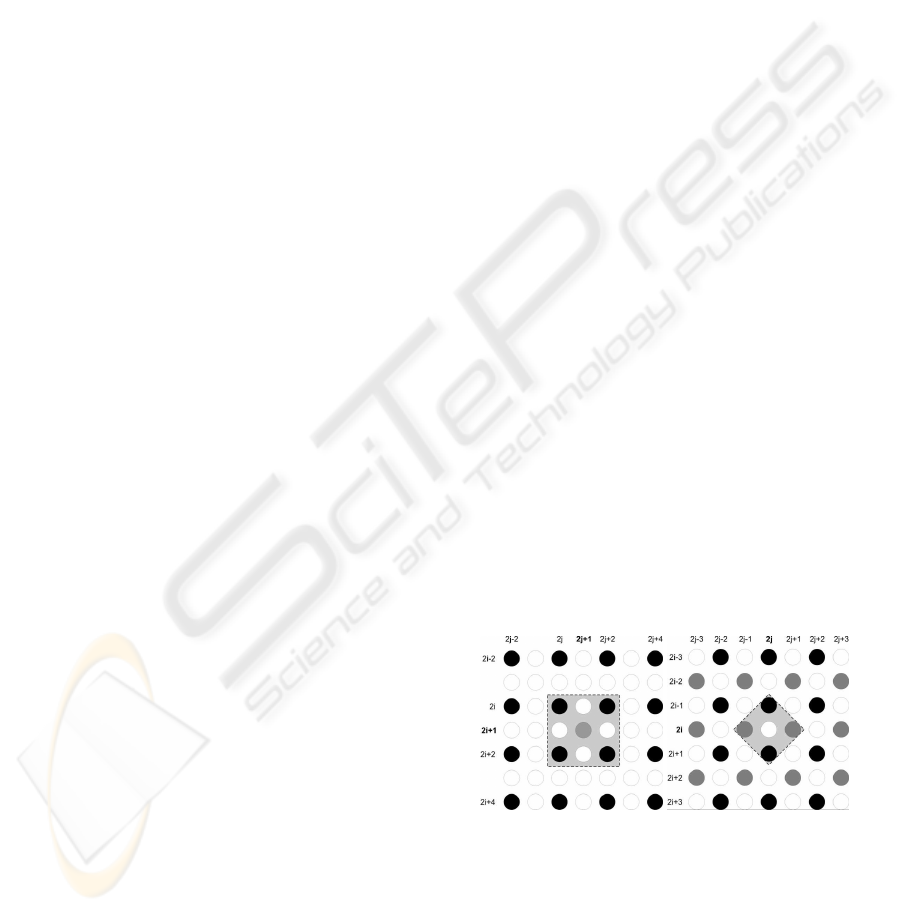
variance. The image is therefore approximately dou-
bled in size by first putting original NxN pixels I
LR
in an enlarged (2N − 1)x(2N − 1) grid I (see Fig. 1)
and then filling in two steps the missing values as
weighted averages of the four closest valued pixels.
Fig. 1 show the first step, inserting the new values in
positions 2i+ 1,2j+ 1, with the formula:
I
2i+1,2j+1
=
~
α· (I
2i,2j
,I
2i,2j+2
,I
2i+2,2j
,I
2i+2,2j+2
).
(1)
The second step fills the remaining gaps in the same
way after a 45 degrees rotation of the grid (Fig. 2).
Figure 1: The two step NEDI interpolation. Original NxN
pixel are placed in a 2N-1x2N-1 grid. Pixels at odd po-
sitions (2i+1,2j+1) are then filled with the NEDI method
(left) as weighted sums of the 4 diagonal neighbors. The
remaining empty pixels are then filled in the same way after
a 45
O
rotation of the grid.
The coefficient of the linear interpolation are the
elements of the vector
~
α = (α
0
,α
1
,α
2
,α
3
) (Fig. 2).
ACCURACY IMPROVEMENTS AND ARTIFACTS REMOVAL IN EDGE BASED IMAGE INTERPOLATION
59
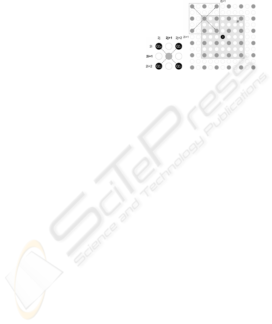
NEDI estimate these α
i
by solving an unconstrained
system of linear equations. The system is obtained
by assuming that the coefficients linking each pixel
with its four diagonal neighbors do not change with
scale (i.e. the relationship is maintained on subsam-
pled/upscaled images) and that they are constant in
a squared window W centered in the interested pixel
location. Fig. 2 shows an example: assuming that
each valued pixel (painted in gray) of the 4x4 (7x7
in the upscaled image) pixel window W centered in
~x = (2i+1,2j+ 1) can be obtained as a weighted sum
of the diagonal neighbors with equal weights, we can
write a system of equations:
C
~
α =~y (2)
where
C =
I
h
1
−1,k
1
−1
I
h
1
−1,k
1
+1
I
h
1
+1,k
1
−1
I
h
1
+1,k
1
+1
I
h
2
−1,k
2
−1
I
h
2
−1,k
2
+1
I
h
2
+1,k
2
−1
I
h
2
+1,K
2
+1
... ... ... ...
... ... ... ...
I
h
N
−1,k
N
−1
I
h
N
−1,k
N
+1
I
h
N
+1,k
N
−1
I
h
N
+1,k
N
+1
h,k ∈ W(2i+ 1,2 j + 1)
and ~y = (I
h
1
,k
1
,I
h
2
,k
2
,I
h
3
,k
3
,..., I
h
N
,k
N
)
T
.
W(2i + 1, 2j + 1) is the set of valued pixels in
the squared window centered in (2i + 1, 2j + 1)
(i.e. the light gray area of Fig. 2). (h
n
,k
n
) are the
coordinates of the n
th
pixel inside the window. The
system is solved by a least squares method to obtain
the α
i
coefficients.
4 LIMITS OF NEDI ALGORITHM
AND SOLUTIONS PROPOSED
(INEDI)
The NEDI technique provides good results due to the
fact that it adapts locally at each resolution the in-
terpolating surface assuming local regularity in cur-
vature. The assumption of local stationarity of the
covariance is violated in several cases and the anal-
ysis of these cases can be exploited to improve the
interpolation results. The use of large and squared
windows to generate the over-constrained system (2)
causes errors and artifacts due to high frequencycom-
ponents and that can be only partially removed by set-
ting thresholds on the residual of the coefficient com-
putation or by using robustestimators. Indeed, the use
of generic robust estimators does not remove artifacts,
because they may introduce non local effects and ad
hoc strategies should be applied.
Figure 2: In the NEDI method, the four coefficient used to
compute the interpolated value (left) are computed assum-
ing that in a squared window around the point each pixel of
the low resolution image is related through the same coeffi-
cients to its 4 closest neighbors.
We identified several problems in the original
formulation and proposed some modifications to in-
crease the interpolation accuracy. The final result
is a modified technique, referred in the following as
iNEDI, improved New Edge Directed Interpolation,
implementing all the improvements proposed and that
are summarized in the following subsections.
4.1 Windows Shape
A first minor problem that, however, can be removed
is that the use of squared windows is not optimal be-
cause it can introduce directional artifacts and anyway
makes the algorithm non isotropic. These effects can
be reduced by simply computing the parameters on
approximately circular windows (except, in our case,
for the pixels excluded by the edge segmentation de-
scribed in the following).
4.2 Non Edge Pixels Handling
It is evident that when the four pixels used to calcu-
late the interpolated ones have a similar gray level,
there is no need to compute the NEDI coefficients, if
the covariance is stationary, a small error causes a bad
conditioningof the solution, even if, on the other hand
the use of linear interpolation changes slightly the re-
sults. This problem is already handled in the original
NEDI formulation, moving to bilinear interpolation if
local gray level variation is above a fixed threshold
THR. We adopted a similar solution, but we applied
the bicubic approximation in low frequency regions.
This choice, of course, do not give improvements in
image quality when THR is low. It gives, however,
the possibility of obtaining a good tradeoff between
VISAPP 2008 - International Conference on Computer Vision Theory and Applications
60
edge direction preservation, accuracy and speed us-
ing higher values of the threshold (i.e. using iNEDI
only for strong edges).
4.3 Edge ”Segmentation”
The main problem in the NEDI formulation is how
to ensure that the window used for the estimation be-
longs almost completely to the same ”edge”. For each
point~x in the enlarged grid to be fitted, the ideal win-
dow where points should be inserted in C and~y should
be a connected region including the 4 valued pixel
pixel closest to~x where local curvatures are smoothly
changing. This is a condition that is stronger than the
constant covariance constraint, that does not guaran-
tee the absence of high component frequencies in the
local fit.
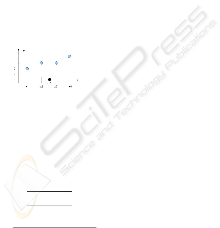
Figure 3: A simple 1D interpolation example showing that
an exact constant covariance interpolation may create com-
pletely wrong results. Assuming that each pixel at the low
resolution can be obtained as a weighted sum of the two
neighbors and assuming weights locally constant, we ob-
tain the black pixel as the one interpolating the profile in
x
5
.
This fact can be shown with a 1D example. Con-
sider the plot of Fig. 3, and suppose we want to
increase the resolution by estimating an interpolated
value in x
5
assuming that I(x
5
) = α
1
I(x
2
) + α
2
I(x
3
)
and that α
1
,α
2
can be estimated from the neighbor-
ing pixels at the coarse scale I(x
1
),I(x
2
),I(x
3
),I(x
4
).
Assuming I(x
2
) = α
1
I(x
1
) + α
2
I(x
3
) and I(x
3
) =
α
1
I(x
2
) + α
2
I(x
4
), the exact solution is:
α
1
=
I(x
2
)I(x
4
) − I(x
3
)
2
I(x
1
)I(x
4
) − I(x
3
)I(x
2
)
α
2
=
I(x
1
)I(x
3
) − I(x
2
)
2
I(x
1
)I(x
4
) − I(x
3
)I(x
2
)
(3)
leading to an interpolated value of:
I(x
5
) =
I(x
2
)
2
I(x
4
) − I(x
3
)
2
I(x
2
) − I(x
2
)
2
I(x
3
) + I(x
3
)
2
I(x
1
)
I(x
1
)I(x
4
) − I(x
3
)I(x
2
)
(4)
With the example values of Fig. 3, with a large vari-
ation in local curvature, we have an ”exact” constant
covariance based interpolation between with an ab-
surd high frequency. This problem is usually less rel-
evant if we have a least squares formulation with sev-
eral independent conditions and the profile is locally
smooth. It is clear, however, that the low value of the
residual of the best fit cannot be used as the unique
condition to determine if the α coefficients computed
with NEDI are reasonable. This is why we decided to
perform an a priori segmentation of the edge region
around the interested point and to control and possi-
bly reject a posteriori the interpolated values in case
of too high frequencies.
To segment the connected ”edge region”, we used
a sort of region growing method defined as follows:
-Start from 4 valued neighboring pixels of the cen-
tral point and add iteratively neighbors(in the original
grid) of these pixels with the following properties:
• The gray level between the maximum and the
minimum value of the 4 neighbors is not lesser
than THR (as in the central point).
• The gray level of each pixel is not larger than the
maximum value of the gray level of the 4 neigh-
bors of the central incremented by a threshold
MARGIN and not lower than the minimum of the
4 neighbors of the central point decremented by
the same MARGIN.
• The Euclidean distance between the pixel and the
central point is less than r.
-Enlarge the ”edge” region with the same rules by in-
creasing r up to a maximum value R if the increment
of the radius correspond to a decrement if the normal-
ized residual of the least squares fit.
With this selective procedure and the control on
the residual, we increase the probability of obtaining
a good interpolation, but there is still the possibility
of having unwanted high frequencies (that are not ex-
cluded by the constant covariance condition and may
occur in case of a small number of samples in the fit).
For this reason we put a further constraint by replac-
ing any interpolated value outside the intensity range
of the four neighbors with the closest of the values
delimiting that range (i.e. maximum or minimum).
4.4 Matrix Conditioning and Error
Propagation
Also when clearly bad regions are eliminated with the
”edge segmentation” procedure, the overconstrained
system (2) is often poorly conditioned and a small er-
ror in ~y can cause a large error in the estimated
ˆ
α.
The sensitivity of the solution to the bad conditioning
depends on the relative error on data. A simple trick
to improve the solution accuracy is to add a constant
ACCURACY IMPROVEMENTS AND ARTIFACTS REMOVAL IN EDGE BASED IMAGE INTERPOLATION
61

value to the gray levels, in order to have all values far
from zero. This simple change is effective in reducing
artifacts and wrong estimates.
Another issue that should be considered is that
for a typical edge we have that the signal is chang-
ing along a fixed direction with constant curvature. In
this case the overconstrained system is clearly badly
conditioned due to the rank deficiency of the problem
(the expected rank of the matrix is 2 and not 4.). This
means that the problem of bad conditioning is almost
always verified and that rejecting neighborhood with
bad condition numbers would result in dropping the
NEDI method almost everywhere.
The fact that C is rank deficient, means that the so-
lution to the least squares problem is not unique, i.e.
there are many vectors
~
α
∗
that minimize ||C
~
α−~y||
2
.
We can therefore look for a reliable choice among the
infinite number of possible solutions.
A method that is often used to find an unique so-
lution is to select the minimum norm solution, that
is obtained through the computation of the Moore-
Penrose pseudo inverse. If we assume that the lo-
cal four pixel configuration is the sum of a term ex-
actly modeled by the constant covariance model plus
an error term (i.e., for an odd point in the first step:
~
I
4
= (I
2i,2j
,I
2i,2j+2
,I
2i+2,2j
,I
2i+2,2j+2
) =
~
I
0
+
~
I
err
), the
squared error on the interpolated value I
2i+1,2j+1
=
~
α
∗
·
~
I
4
is (
~
α
∗
·
~
I
err
)
2
and it is in general lowered by
choosing the minimum norm solution for α
∗
. We
solved therefore the overconstrainedsystem using this
method.
4.5 Global Brightness Invariance
With the NEDI method, interpolated pixel values
change with the global brightness, i.e. they do not
depend only on differences between neighboring
values, but also on the absolute value. This effect can
be easily removed by changing the NEDI constraint
by subtracting the average of the four neighbors
intensities from the values inserted in C and ~y, i.e.
replacing C with
C
′
=
I
h
1
−1,k
1
−1
−
¯
I
h
1
,k
1
I
h
1
−1,k
1
+1
−
¯
I
h
1
,k
1
... ...
I
h
2
−1,k
2
−1
−
¯
I
h
2
,k
2
I
h
2
−1,k
2
+1
−
¯
I
h
2
,k
2
... ...
... ... ... ...
... ... ... ...
I
h
N
−1,k
N
−1
−
¯
I
h
N
,k
N
I
h
N
−1,k
N
+1
−
¯
I
h
N
,k
N
... ...
h,k ∈ W(i, j)
and~y with
~
y
′
= (I
h
1
,k
1
−
¯
I
h
1
,k
1
,I
h
2
,k
2
−
¯
I
h
2
,k
2
,..., I
h
N
,k
N
−
¯
I
h
N
,k
N
)
T
where
¯
I
h,k
=
(I
h
1
−1,k
1
−1
+I
h
1
−1,k
1
+1
+I
h
1
+1,k
1
−1
+I
h
1
+1,k
1
+1
)
4
.
I(i, j) is then clearly obtained as:
I(i, j) = α
′
· (I
i−1, j−1
,I
i−1, j+1
,I
i+1, j−1
,I
i+1, j+1
) +
¯
I
i, j
.
This change clearly makes the matrix C
′
rank
deficient, but, as discussed before, the solution is
still possible with the pseudo-inverse. Experimental
results show, however, that the advantages obtained
in the interpolation of natural images in this way is
small.
5 EXPERIMENTAL RESULTS
The modified technique described has been widely
tested and compared with other methods found in lit-
erature as well as with the original NEDI. The new
method has been has been implemented in Matlab
and the code is publicly available at the web site
http://inedi.tecnick.com. We have also coded and
tested other methods (Chen’s and Isophote based)
while for the linear methods we used the basic image
processing Matlab functions. The NEDI implementa-
tion used is the original Matlab code kindly provided
to us by prof. Xin Li.
5.1 Enlarged Subsampled Images
A simple test often used in literature to measure quan-
titatively the interpolation accuracy consists of gener-
ating low resolution images by filtering and subsam-
pling high resolution ones and then measure the dif-
ference between the differently re-upsized images and
the original one. The measure used to compute this
difference is mainly the Peak Signal to Noise Ratio,
defined as:
PSNR = 20log
10
MAXPIX
∑
W
i=1
∑
H
j=1
(I
exp
(i, j)−I
orig
(i, j))
2
(W∗H)
(5)
where I
exp
(i, j) is the zoomed subsampled image,
I
orig
the original one, W and H the image dimensions
and MAXPIX the end scale value of the pixel inten-
sity. The value measures therefore how much the in-
terpolation method is able to guess the correct im-
age values at unknown locations for each particular
scene/image considered.
Due to the fact that the method is strongly depen-
dent on the scene and on the imaging procedure, it
is necessary to test the results on a relevant set of
images and/or on complex images representing dif-
ferent natural textures. We performed our tests on
VISAPP 2008 - International Conference on Computer Vision Theory and Applications
62
an original set of 9 1025x1025 images, transformed
in low resolution ones (256x256 and 128x128) and
then upscaled (2x,4x) with different algorithms. Im-
ages (see Fig. 4) are all natural and present a great
variety of textures and local frequencies. Note that
the (511x511 or 512x512) reference images used to
compute the PSNR are different for different inter-
polation algorithms due to the different image shifts
introduced by the various technique. An half pixel
image shift not compensated may compromise the
correctness of the comparison and lead to a wrong
estimate of algorithms performances. Tables 1 and
2 show the PSNR values for each image obtained
with NEDI and iNEDI algorithms and other selected
techniques (bilinear and bicubic, an iterative method
based on isophote smoothing based on (Morse and
Schwartzwald, 2001) and the fast edge based method
describedin (Chen et al., 2005) for 2x and 4x enlarge-
ment. It is evident that the improvements proposed
give a relevant increase in the measured quality of
NEDI and that the accuracy of the reconstruction is
higher than those obtained with the other techniques.
Figure 4: Images used for the quantitative comparison.
One fact that may appear surprising is that the per-
formances of the original NEDI and of the other two
literature algorithm presented are worse than the re-
sults of the bicubic interpolation. Our comparison
was performed carefully, using the bicubic approxi-
mation implemented in MATLAB, the original Xin Li
implementation for original NEDI and following the
algorithms description of other authors. The parame-
ters used were chosen with a trial and error method in
order to minimize the reconstruction error.
It should be considered, however, that the good re-
sults of the bicubic interpolation does not mean that
it is surely better than other methods: original NEDI,
as well as the other edge based method tested (Chen,
Isophote), are effective in removing the typical ar-
tifacts of the bicubic and bilinear interpolation (i.e.
jagged contours). The lower PSNR is probably due to
the other kinds of artifacts affecting NEDI and exces-
sive smoothing of the other approaches.
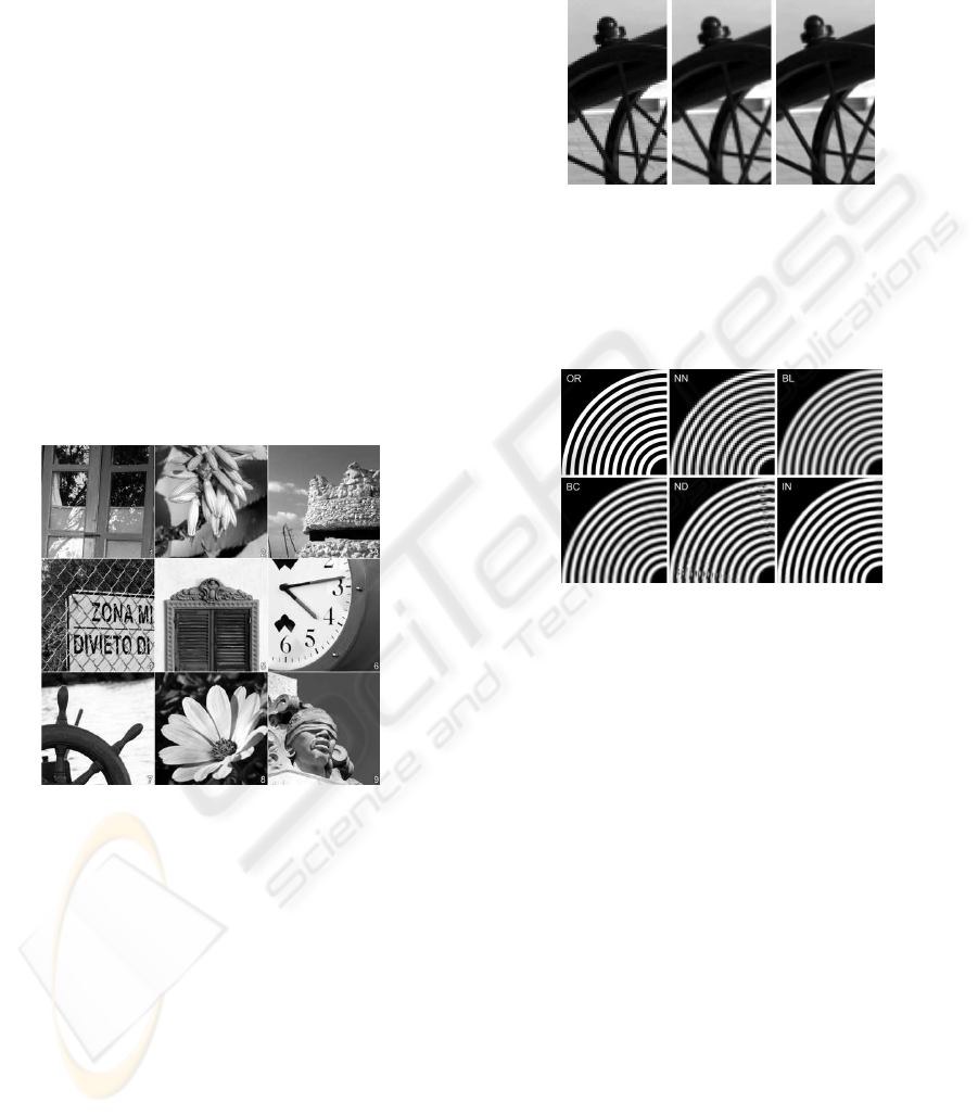
Figure 5: 8X enlarged images. Jagged contours are evident
in nearest neighbor and bicubic interpolation (left, center).
The NEDI interpolation (right), present sharp edges, even if
introduces different artifacts and perform often worser than
the bicubic method in quantitative comparisons. Our im-
provements to the method reduce evidently these effects.
Figure 6: Original artificial image (OR) and 8X
reduced/enlarged images (NN=Nearest Neighbor,
BL=Bilinear interpolation, BC=Bicubic interpolation,
ND=Nedi, IN=iNedi). The NEDI interpolation removes
jagged contours, but introduces directional artifacts. iNedi
modifications remove these effects.
We also performed a test on an artificial image to
show the improvements of iNEDI over NEDI in the
removal of directional artifacts. Fig.6 shows an orig-
inal b&w image with concentric circles and the sub-
sampled and 8x enlarged versions obtained with pixel
replication, bilinear, bicubic, NEDI and iNEDI inter-
polations. INEDI clearly removes not only the jagged
lines effects of the linear methods, but also removes
the directional artifacts of NEDI. The PSNR value is
increased by more than 3 dB.
To compare the iNEDI technique with other
techniques available on commercial software, we
also tested the implemented method on a test im-
age provided on the internet site http://www.general-
cathexis.com/interpolation.html where several inter-
polation methods implemented on the SAR Image
Processor package are compared. The iNEDI algo-
rithm provided a PSNR relevantly higher (1dB) than
the best one in the reported comparison (see Table 3).
ACCURACY IMPROVEMENTS AND ARTIFACTS REMOVAL IN EDGE BASED IMAGE INTERPOLATION
63
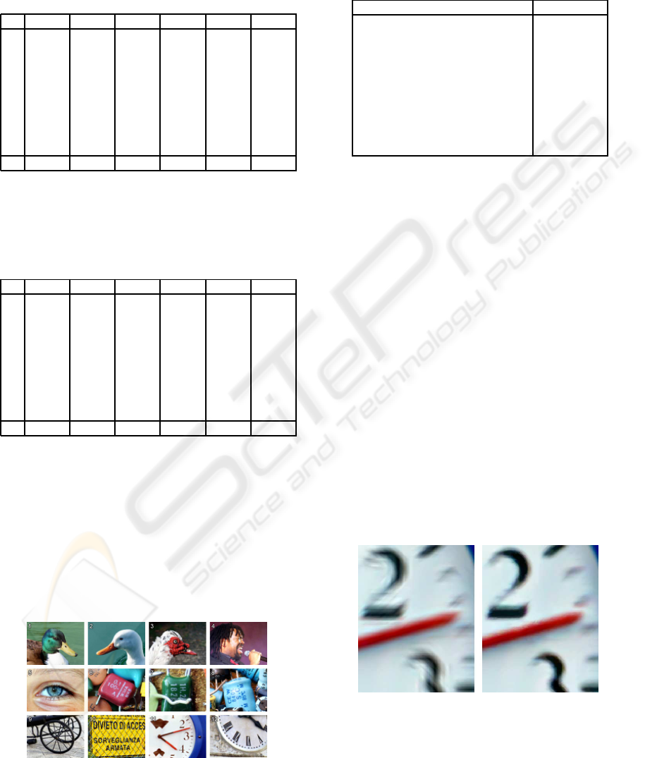
Table 1: PSNR values (dB) obtained on 2x enlarged images
with different methods. The modified edge directed inter-
polation obtained an average increment of 0.85 dB on the
original Xin Li technique and is clearly superior to all the
other methods.
Im iNEDI NEDI Bicub. Bilin. Chen Isoph.
1 30.22 29.58 30.42 28.88 29.19 29.05
2 38.10 37.33 37.81 35.27 36.33 36.27
3 29.45 28.64 29.91 28.23 28.41 27.91
4 29.10 27.47 28.27 25.80 26.82 27.02
5 32.95 31.98 33.48 31.36 31.72 32.10
6 33.68 32.57 32.15 30.30 31.50 32.26
7 37.46 36.92 36.33 34.38 35.75 36.54
8 36.78 36.21 36.20 33.68 34.95 35.49
9 34.77 34.11 34.40 32.56 33.55 33.76
Av 33.61 32.76 33.22 31.16 32.02 32.27
Table 2: PSNR values (dB) obtained on 4x enlarged images
with different methods. The modified edge directed inter-
polation obtained an average increment of 0.85 dB on the
original Xin Li technique and is clearly superior to all the
other methods.
Im iNEDI NEDI Bicub Bilin Chen Isoph
1 24.77 24.21 24.76 24.10 23.98 23.82
2 30.10 29.42 29.70 28.37 28.53 28.52
3 23.80 23.22 23.89 23.16 22.88 22.50
4 21.30 19.95 20.71 19.62 19.64 19.63
5 25.90 25.38 26.11 25.22 25.11 24.96
6 27.10 25.69 25.79 24.72 25.04 25.34
7 30.70 30.04 29.68 28.44 29.12 29.90
8 29.24 28.31 28.27 26.85 27.32 27.89
9 28.68 27.73 28.02 26.91 27.18 27.34
Av 26.84 25.99 26.33 25.27 25.42 25.54
5.2 Qualitative Scores
A group of 24 people have been asked to give a ”qual-
itative” judgment on 12 color images originally of
80x60 pixels and enlarged (independently for each
color channel) of a factor 8 with iNEDI and NEDI
algorithms as well as with bicubic and bilinear inter-
polation.
Figure 7: Color images used for the qualitative comparison
(Results in Table 4).
Table 3: PSNR obtained with the proposed iNEDI al-
gorithm on a test image compared with the results of
several methods reported on the site http://www.general-
cathexis.com/interpolation.html.
Method PSNR [dB]
iNEDI 29.65
DDL with SuperRez Postproc. 28.65
LAD Deconvolution 28.57
Pseudonverse with SR Postproc. 28.57
Jensen Zhao Xin Li 27.90
Zhao Xin Li 27.65
Bicubic 27.49
Triangulation 27.10
Bilinear 26.92
Nearest neighbor 26.19
The qualitativejudgmenthas been performed sort-
ing the images from the worst (1) to the best (4).
The qualitative test is really important in choosing
an optimal algorithm because the main application
of this kind of algorithm consists in the improve-
ment of the perceived image quality in printing or im-
age display applications. The results obtained (Ta-
ble 4) confirmed the results of the analysis based on
the PSNR. In fact, the original NEDI score is lower
than that obtained with the bicubic approximation.
This is due to the relevant artifacts of the technique,
that preserves well discontinuities and creates sharp
edges, but also creates evident ”oil painting” artifacts
that makes the image unnatural. This problem is re-
vealed by an higher reconstruction error, but appear
also clear to the human eye. The edge segmentation of
the iNEDI method reduces relevantly these artifacts,
creating natural images still more similar to real high
resolution photos than those obtained with bicubic in-
terpolation.
Figure 8: Artifacts reduction obtained with the iNEDI
method(right) with respect to NEDI (left): non local effects
are clearly reduced by adapting window shapes and size,
discarding high frequency interpolated values and optimiz-
ing the least squares procedure.
VISAPP 2008 - International Conference on Computer Vision Theory and Applications
64

Table 4: Average position (1-4) in a qualitative comparison
performed by 24 subjects on 12 images enlarged (8x) with
different methods.
Im. iNEDI NEDI BicubicBilinear
1 3.75 2.92 2.13 1.21
2 4.00 2.83 2.00 1.17
3 3.96 2.25 2.54 1.25
4 3.75 2.29 2.67 1.29
5 3.58 2.42 2.67 1.33
6 3.96 2.04 2.63 1.38
7 3.79 2.00 2.88 1.33
8 3.83 1.88 2.96 1.33
9 3.75 2.29 2.75 1.21
10 3.79 1.71 3.08 1.42
11 3.88 2.08 2.75 1.29
12 3.75 2.29 2.67 1.29
Avg. 3.82 2.25 2.64 1.29
6 DISCUSSION
We presented an analysis of popular methods to en-
large natural images without any additional informa-
tion and several subjective and objective experimen-
tal tests comparing the performances of different al-
gorithms. In particular, we introduced and motivated
several improvements to the well known Li and Or-
chard’s NEDI method, obtaining a new algorithm,
iNEDI, that provides the best results among all the
tested methods, even if at the cost of a huge compu-
tational complexity. Images enlarged with the pro-
posed technique appear, in fact, more natural and less
smoothed than those obtained with other approaches
presented in literature and both psychological and
quantitative tests measuring differences between en-
larged subsampled photos and original ones confirm
this fact. For selected applications (i.e. printing or
off line extrapolation of high resolution textures from
low resolution data) the relevant computational effort
is not a problem, while for applications requiring a
fast image processing (i.e. improving quality of video
streaming), different methods should be applied, even
if the algorithm can be optimized and parallelized. We
are currently investigating new edge based methods
that seem to provide similar results with relevantly
low computational complexity.
ACKNOWLEDGEMENTS
Thanks to prof. X. Li for kindly providing the origi-
nal NEDI code and to Alan L. Scheinine for checking
the English. This work was partially supported by the
Italian Ministry of University and Scientific Research
Grant PRIN 2006010149 003 (3Shirt).
REFERENCES
Atkins, C. B., Bouman, C. A., and Allebach, J. P. (2001).
Optimal image scaling using pixel classification. In
Proc. IEEE Int. Conf. Image Processing, volume 3,
pages 864–867.
Battiato, S., Gallo, G., and Stanco, F. (2002). A locally-
adaptive zooming algorithm for digital images. Image
and Vision Computing.
Cha, Y. and Kim, S. (2007). The error-amended sharp edge
(ease) scheme for image zooming. IEEE Transactions
on Image Processing, 16:1496–1505.
Chen, M., Huang, C., and Lee, W. (2005). A fast edge-
oriented algorithm for image interpolation. Image and
Vision Computing, 23:791–798.
Freeman, W. T., Jones, T. R., and Pasztor, E. C. (2002).
Example-based super-resolution. IEEE Computer
Graphics and Applications, 22(2):56–65.
Li, X. and Orchard, M. T. (2001). New edge-directed inter-
polation. IEEE Trans. on Image Processing, 10:1521–
1527.
Lu, X., Hong, P. S., and Smith, M. J. T. (2003). An effi-
cient directional image interpolation method. In Proc.
IEEE Int. Conf. Acoustics Speech Signal Processing,
volume 3, pages 97–100.
Morse, B. and Schwartzwald, D. (2001). Image mag-
nification using level-set reconstruction. In Proc.
IEEE Conf. Computer Vision Pattern Recognition,
volume 3, pages 333–340.
Muresan, D. and Parks, T. (2004). Adaptively quadratic
(aqua) image interpolation. IEEE Transactions on Im-
age Processing, 13(5):690–698.
Schultz, R. R. and Stevenson, R. L. (1994). A bayesian
approach to image expansion for improved definition.
IEEE Trans. Image Processing, 3:233–242.
Su, D. and Willis, P. (2004). Image interpolation by pixel
level data-dependent triangulation. Computer Graph-
ics Forum, 23.
Sun, J., Zheng, N., Tao, H., and Shum, H. (2003). Im-
age hallucination with primal sketch priors. In Pro-
ceedings IEEE conf. on Computer Vision and Pattern
Recognition, volume 2.
Takahashi, Y. and Taguchi, A. (2002). An enlargement
method of digital images with the prediction of high-
frequency components. In Proc. IEEE Int. Conf. Ac.
Speech Signal Proc., volume 4, pages 3700–3703.
Wang, Q. and Ward, R. K. (2007). A new orientation-
adaptive interpolation method. IEEE Transactions on
Image Processing, 16:889–900.
ACCURACY IMPROVEMENTS AND ARTIFACTS REMOVAL IN EDGE BASED IMAGE INTERPOLATION
65
