MULTIPLE VIEW GEOMETRY FOR MIXED DIMENSIONAL

CAMERAS

Kazuki Kozuka and Jun Sato

Department of Computer Science and Engineering, Nagoya Institute of Technology

Nagoya, 466-8555, Japan

Keywords:

Multiple view geometry, stereo vision, structure from motion, non-homogeneous cameras.

Abstract:

In this paper, we analyze the multiple view geometry under the case where various dimensional imaging

sensors are used together. Although the multiple view geometry has been studied extensively and extended

for more general situations, all the existing multiple view geometries assume that the scene is observed by the

same dimensional imaging sensors, such as 2D cameras. In this paper, we show that there exist multilinear

constraints on image coordinates, even if the dimensions of camera images are different each other. The new

multilinear constraints can be used for describing the geometric relationships between 1D line sensors, 2D

cameras, 3D range sensors etc., and for calibrating mixed sensor systems.

1 INTRODUCTION

The multiple view geometry is very important for de-

scribing the relationship between images taken from

multiple cameras and for recovering 3D geometry

from images (Hartley and Zisserman, 2000; Faugeras

and Luong, 2001). The traditional multiple view ge-

ometry assumes the projection from the 3D space

to 2D images (Faugeras and Keriven, 1995; Triggs,

1995; Heyden, 1998; Hartley and Zisserman, 2000).

As a result, the traditional multiple view geometry is

limited for describing the case, where enough num-

ber of corresponding points are visible from a static

conﬁguration of multiple cameras. Recently, some

efforts for extending the multiple view geometry for

more general point-camera conﬁgurations have been

made (Hartley and Schaffalitzky, 2004; Shashua and

Wolf, 2000; Sturm, 2005; Wexler and Shashua, 2000;

Wolf and Shashua, 2001). Wolf et al. (Wolf and

Shashua, 2001) studied the multiple view geometry

on the projections from N dimensional space to 2D

images and showed that it can be used for describing

the relationship of multiple views obtained from mov-

ing cameras and moving points with constant speed.

Hayakawa et al. (Hayakawa and Sato, 2006) showed

that it is possible to deﬁne multilinear relationships

for general non-rigid motions.

However, these existing research works assume

that the scene is observed by homogeneous multiple

cameras, that is the dimensions of images of multiple

cameras are the same. Since it is sometimes impor-

tant to combine different type of sensors, such as line

sensors, 3D range sensors and cameras, the assump-

tion of homogeneous cameras is the big disadvantage

of the existing multiple view geometry. On the other

hand, the traditional multiple view geometry has been

extended gradually for non-homogeoneous sensors.

Sturm (Sturm, 2002) analyzed a method for mixing

catadioptric cameras and perspective cameras, and

showed that the multilinear relationship between stan-

dard perspective cameras and catadioptric cameras

can be described by non-square tensors. Thirthala et

al. (Thirthala and Pollefeys, 2005) analyzed the tri-

linear relationship between a perspective camera and

two 1D radial cameras for describing the relationship

between standarad cameras and catadioptric cameras.

Although these results show some posibility of the

use of non-homogeneous sensors, these are limited

for speciﬁc camera combinations.

Thus, we in this paper analyze the multiple view

geometry for general mixed dimensional cameras in

various dimensional space, and show the multilin-

ear relationships for various combinations of non-

homogeneous cameras. We also show that these mul-

Kozuka K. and Sato J. (2008).

MULTIPLE VIEW GEOMETRY FOR MIXED DIMENSIONAL CAMERAS.

In Proceedings of the Third International Conference on Computer Vision Theory and Applications, pages 5-12

DOI: 10.5220/0001072500050012

 SciTePress

tilinear relationships can be used for calibrating mul-

tiple dimensional cameras and for transfering corre-

sponding points to different dimensional cameras.

2 PROJECTION FROM P

TO P

Let us consider a projective camera P which projects

a point X in the kD projective space to a point x in the

nD projective space.

x ∼ PX (1)

where, ∼ denotes equality up to a scale. The camera

matrix, P, of this camera is (n+ 1) × (k+ 1) and has

((k+ 1) × (n+ 1) − 1) DOF.

3 MULTIPLE VIEW GEOMETRY

OF MIXED DIMENSIONAL

CAMERAS

We next consider the properties of the multiple view

geometry of mixed dimensional cameras, which rep-

resent geometric relationships of multiple cameras

with various dimensions. Let us consider kD pro-

jective space, P

, and a set of various dimensional

cameras in the space. Consider k types of cameras

(i = 1, ··· , k) which induce projections from P

(i = 1, ··· , k) respectively. For example, C

type

cameras project a point in P

to a point in P

, and C

type cameras project a point in P

to a point in P

Suppose there are n

cameras of type C

(i = 1, ··· , k)

in the kD space. Then, we have totally N =

∑

i=1

cameras in the kD space. In this paper, a set of these

cameras is represented by a k dimensional vector, n,

as follows:

n = [n

, n

, ··· , n

]

⊤

(2)

Now, we consider DOF of N view geometry of

mixed dimensional cameras, and specify the number

of points required for computing the N view geometry

of mixed dimensional cameras. Since camera matri-

ces from P

to P

are (k + 1) × (i+ 1), the DOF of N

cameras is N((k + 1)(i + 1) − 1). The kD homogra-

phy is represented by (k+ 1) × (k +1) matirx, and so

it has (k+ 1)

− 1 DOF. Since these N cameras are in

a single kD projective space, the total DOF of these N

cameras is as follows:

L =

∑

i=1

((k+ 1)(i+ 1)− 1) − (k + 1)

+ 1 (3)

= (k+1)(n

⊤

i− k) + kN −k (4)

where, i = [1, 2, ··· , k]

⊤

. Thus, the N view geometry

of mixed dimensional cameras has L DOF. The very

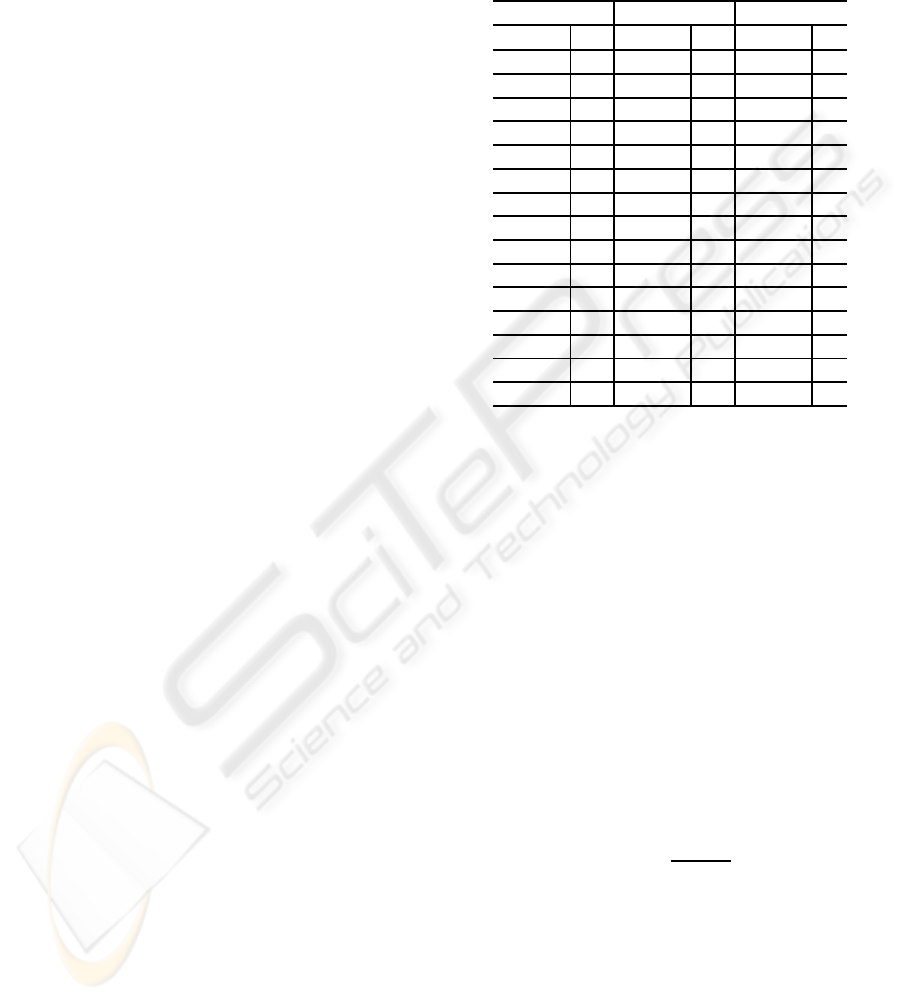
Table 1: The minimum number of corresponding points re-

quired for computing the multiple view geometry of mixed

dimensional cameras in the 3D space. Note, the multiple

view geometries of n

⊤

= [3, 0, 0], [2, 0, 0] and [1, 1, 0] do not

exist, since the image information is not enough for deﬁning

the multiple view geometry in these cases.

4 Views 3 Views 2 Views

⊤

# n

⊤

# n

⊤

[4,0,0] 13 [2,1,0] 10 [0,2,0] 7

[3,1,0] 9 [1,2,0] 7 [1,0,1] 7

[2,2,0] 7 [0,3,0] 6 [0,1,1] 6

[1,3,0] 7 [2,0,1] 7 [0,0,2] 5

[0,4,0] 6 [1,1,1] 6

[3,0,1] 7 [0,2,1] 6

[2,1,1] 7 [1,0,2] 6

[1,2,1] 6 [0,1,2] 6

[0,3,1] 6 [0,0,3] 5

[2,0,2] 6

[1,1,2] 6

[0,2,2] 6

[1,0,3] 6

[0,1,3] 6

[0,0,4] 5

special case of the multiple view geometry of mixed

dimensional cameras is the traditional multiple view

geometry of 2D cameras which induce projections

from P

to P

. In this case, k = 3 and n = [0, 2, 0]

⊤

Suppose M points in the kD space are projected

to these N cameras. Then we have image informa-

tion with Mn

⊤

i DOF from these cameras. Thus, the

following inequality must hold for ﬁxing all the ge-

ometry of N cameras and M points in the kD space.

⊤

i ≥ L+ kM (5)

By substituting (4) into (5), we ﬁnd that the following

condition must hold for computing the multiple view

geometry of mixed dimensional cameras.

M ≥ k + 1+

kN − k

⊤

i− k

(6)

(6) shows the minimum number of corresponding

points required for computing the multiple view ge-

ometry of mixed dimensional cameras.

The complete table of the minimum number of

corresponding points for mixed dimensional cameras

in the 3D space is as shown in table 1.

In the following part of this paper, we show the

detail of the multiple view geometry of some example

combinations of different dimensional cameras.

VISAPP 2008 - International Conference on Computer Vision Theory and Applications

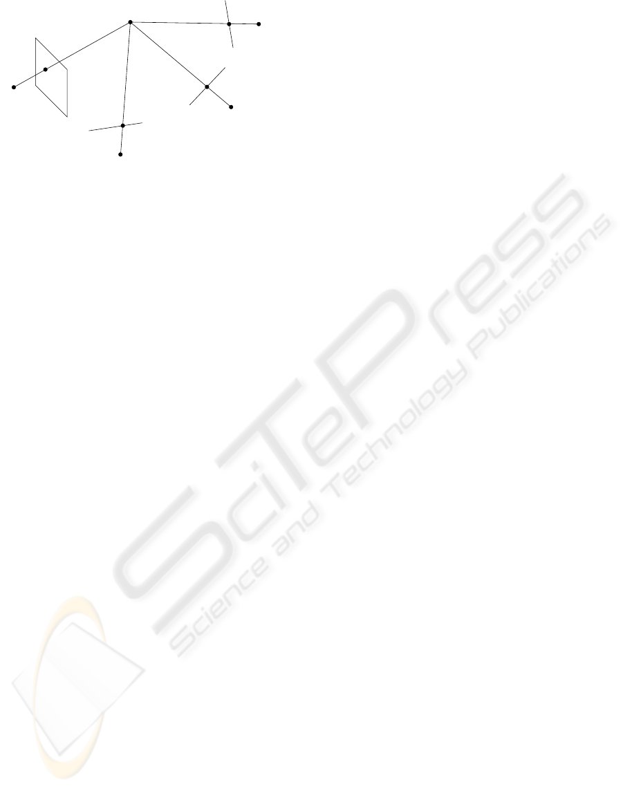
Figure 1: N view geometry of a 2D camera C

and N − 1

1D cameras C

(i = 1, ··· , N − 1).

4 N VIEW GEOMETRY OF

n = [N − 1, 1, 0]

⊤

In this section, we consider the N view geometry

of n = [N − 1, 1, 0]

⊤

, i.e. a single 2D camera and

(N − 1) 1D cameras and no 3D camera in the 3D

space. Let a 3D point X = [X

, X

]

⊤

be pro-

jected to x = [x

, x

]

⊤

in a 2D camera C

, and let

X be projected to v

= [v

, v

]

⊤

in 1D line cameras C

(i = 1, ··· , N − 1) as shown in Fig. 1. These projec-

tions can be described by using the camera matrices

of C

and P

of C

as follows:

x ∼ P

X (7)

∼ P

X (i = 1, ··· , N − 1) (8)

where, P

is a 3× 4 matrix and P

are 2 × 4 matrices

respectively. By reformulating (7) and (8), we have

the following equation for X:







N−1













N−1



















(9)

where, λ denotes a scalar. Extracting the (N + 4) ×

(N + 4) sub-square matrix M of the left most matrix

in (9), and computing the determinant of M, we have

the following multilinear constraints of mixed dimen-

sional cameras:

detM = 0 (10)

By expanding (10) in 3 views and 4 views, we have

the following trilinear constraints and quadrilinear

constraints respectively:

= 0 (11)

iam

abcd

= 0

(12)

where the indices i, a and m take 1 through 3, and all

the other indices take 1 or 2 in (11) and (12). The

tensor ε

ijk

takes 1 if {i, j, k} is even permutation, and

it takes −1 if {i, j, k} is odd permutation. Similarly,

the tensor ε

takes 1 if {i, j} is even permutation, and

it takes −1 if {i, j} is odd permutation.

The 3× 2× 2 tensor T

is the trifocal tensor, and

the 3× 2× 2× 2 tensor Q

abcd

is the quadrifocal ten-

sor of the mixed dimensional cameras. Note there is

no 2 view geometry in this case, since the combina-

tion of a 2D camera and a 1D line camera does not

have enough information for deﬁning the 2 view con-

straints. Also, there is no linear constraint for more

than 4 views.

By substituting n = [N − 1, 1, 0]

⊤

and k = 3 into

(4), we ﬁnd that the N view geometry has 7N − 11

DOF in this case, and therefore the trifocal tensor

T has 10 DOF, and the quadrifocal tensor Q has 17

DOF.

From (6), we ﬁnd that the minimum number of

corresponding points required for computing the tri-

focal tensor T is 10, while the minimum number of

corresponding points for the quadrifocal tensor Q is

We next consider linear estimation of T tensor

and Q tensor. Since T tensor is 3 × 2 × 2, it has 11

unknowns except a scale. On the other hand, a set

of corresponding points in three views provides us a

single constraint for T tensor from (11). Thus, we re-

quire 11 correspondingpoints for computing T tensor

linearly.

Similarly, Q tensor is 3 × 2 × 2 × 2 and has 23

unknowns except a scale. Since (12) provides us

2 linearly independent constraints for Q tensor, we

can compute Q tensor linearly from 12 correspond-

ing points.

Once the trifocal tensor T is obtained, the epipolar

line l

= v

in the 2D image can be com-

puted from v

and v

in 1D images. Similarly, once

the quadrifocal tensor is obtained, the corresponding

point x in the 2D image can be computed from the

points v

, v

and v

in 1D images by using (12).

5 N VIEW GEOMETRY OF

n = [0, N − 1, 1]

⊤

We next consider the N view geometry in the case

where a 3D range sensor and multiple 2D cameras

exist in the 3D space, i.e. k = 3 and n = [0, N− 1, 1]

⊤

Let a 3D point X = [X

, X

]

⊤

be measured

by a 3D range sensor C

, and let y = [y

, y

]

⊤

be the data measured by this sensor as shown in Fig. 2.

MULTIPLE VIEW GEOMETRY FOR MIXED DIMENSIONAL CAMERAS

range sensor

coordinates

world

coordinates

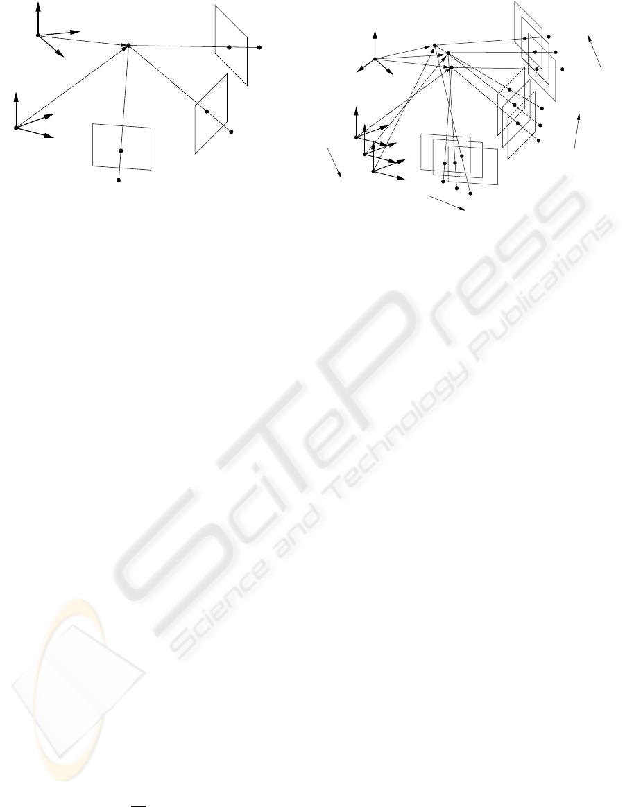
Figure 2: N view geometry of a 3D range sensor C

and

N − 1 2D cameras C

(i = 1, ··· , N −1).

Suppose the point X is also observed by (N − 1) 2D

cameras C

as x

= [x

, x

]

⊤

(i = 1, ··· , N − 1).

Then, the projection in the 3D range sensor and

the 2D cameras can be described as follows:

y ∼ P

X (13)

∼ P

X (i = 1, ··· , N − 1) (14)

where, P

is a 4 × 4 matrix with 15 DOF, and P

3× 4 projection matrices with 11 DOF.

From the similar analysis with section 4, we can

derive the following bilinear, trilinear and quadrilin-

ear constraints for the mixed dimensional cameras:

jbp

= 0

(15)

iamn

jbp

kcq

ambc

= 0

npq

(16)

iamn

jbp

kcq

ldr

abcd

= 0

mnpqr

(17)

where, indices i, a, m and n take 1 through 4, and all

the other indices take 1 through 3 in (15), (16) and

(17). The tensor ε

ijkl

takes 1 if {i, j, k, l} is even per-

mutation, and it takes −1 if {i, j, k, l} is odd permuta-

tion.

The 4 × 3 tensor B

, 4 × 4× 3 × 3 tensor T

ambc

and 4× 3× 3 × 3 tensor Q

abcd

are the bifocal tensor,

trifocal tensor and quadrifocal tensor of the mixed di-

mensional cameras.

By substituting n = [0, N − 1, 1]

⊤

and k = 3 into

(4) we ﬁnd that the N view geometry has 11N − 11

DOF. Thus, B

has 11 DOF, T

ambc

has 22 DOF and

abcd

has 33 DOF respectively. Also, we ﬁnd from

(6) that the following condition must hold for com-

puting B

, T

ambc

and Q

abcd

M ≥

(18)

This means that the minimum number of correspond-

ing points required for computing the multifocal ten-

sors is 6 and is irrespective of the number of cameras.

(t)

(t+1)

(t+2)

range sensor

coordinates

(t+2)

(t)

(t+1)

coordinates

world

(t+1)

(t+2)

(t)

(t+1)

(t+2)

(t+1)

(t)

(t+2)

(t)

(t+1)

(t+2)

(t)

(t+1)

(t+2)

(t)

(t+1)

(t+2)

y(t+1)

y(t+2)

y(t)

Figure 3: N view geometry of a moving 3D range sensor C

and N −1 moving 2D cameras C

(i = 1, ··· , N −1).

We next consider the linear estimation of these

multifocal tensors. The bifocal tensor B

is 4× 3 and

has 11 unknowns except a scale. Since we have 2

linearly independent constraints for B

from (15), 6

corresponding points are enough for computing B

linearly.

6 N VIEW GEOMETRY OF

n = [0, N − 1, 1, 0]

⊤

We next extend the case described in section 5 and

consider the N view geometry of a translational 3D

range sensor and translational 2D cameras as shown

in Fig. 3. If the 3D range sensor and the 2D cam-

eras move independently, the multilinear constraints

described by (15), (16) and (17) no longer hold. How-

ever, if we consider the multiple view geometry in the

higher dimensional space, then we can derivethe mul-

tilinear constraints which describe the relationship be-

tween a moving3D range sensor and moving 2D cam-

eras.

Suppose we have a moving point

X = [X, Y, Z]

⊤

the 3D space, and suppose the point is projected to an

image point

x = [x, y]

⊤

in a 2D camera. If the camera

moves translationally with a constant speed, ∆X, ∆Y

and ∆Z in X, Y and Z directions, we can describe the

relationship between the image point

x and the 3D

point

X as follows:









∼















X −T∆X

Y − T∆Y

Z −T∆Z







(19)

where, T denotes a time. If we consider a 4D space

which consists of X, Y, Z and T, then the projection

described by (19) can be rewritten as follows:

VISAPP 2008 - International Conference on Computer Vision Theory and Applications

∼

−P

∆X−P

∆Y−P

∆Z P

−P

∆X−P

∆Y−P

∆Z P

−P

∆X−P

∆Y−P

∆Z P













(20)

Since the motion of the camera is unknown but

is constant, the 3 × 5 projection matrix in (20) is un-

known but is ﬁxed. This means a moving camera in

the 3D space can be considered as a static camera in

the 4D space.

Similarly, a translational 3D range sensor can be

considered as a static range sensor in the 4D space as

follows:













∼







−P

∆X−P

∆Y−P

∆Z P

−P

∆X−P

∆Y−P

∆Z P

−P

∆X−P

∆Y−P

∆Z P

−P

∆X−P

∆Y−P

∆Z P



















(21)

This means the multiple view constraints between

a moving range sensor and moving cameras can be

deﬁned in the 4D space. Thus, we consider the mul-

tiple view geometry in the case where k = 4 and

n = [0, N − 1, 1, 0]

⊤

Suppose a 4D point, whose homoge-

neous coordinates are represented by W =

, W

]

⊤

, is projected to an image

point in a translational 2D camera, whose homoge-

neous coordinates are represented by x= [x

, x

]

⊤

Suppose the 4D point W is also measured by a trans-

lating 3D range sensor as y = [y

, y

]

⊤

. Then,

the projection in the moving 3D range sensor and the

moving 2D cameras can be described as follows:

y ∼ P

W (22)

∼ P

W (i = 1, ··· , N − 1) (23)

where, P

is a 4 × 5 matrix with 19 DOF, and P

are

3× 5 matrices with 14 DOF.

By deﬁning the matrix M similar to the one in (9)

, and expanding detM = 0, we have the bilinear, tri-

linear, quadrilinear and quintilinear constraints (i.e. 5

view constraints) for the moving cameras and range

sensors as follows:

= 0 (24)

jbr

kcs

= 0

(25)

iapq

jbr

kcs

ldt

apbcd

= 0

qrst

(26)

iapq

jbr

kcs

ldt

meu

abcde

= 0

pqrstu

(27)

where, indices i, a, p, q take 1 through 4, and all

the other indices take 1 through 3. B

, T

, Q

apbcd

and R

abcde

are the bilinear, trilinear quadrilinear and

quintilinear tensors respectively.

By substituting k = 4 and n = [0, N −1, 1, 0]

⊤

into

(4), we ﬁnd that the N view geometry has 14N − 19

DOF, and thus B

, T

, Q

apbcd

and R

abcde

have 9

DOF, 23 DOF, 37 DOF and 51 DOF respectively.

Also, by substituting k = 4 and n = [0, N −

1, 1, 0]

⊤

into (6), we ﬁnd that the minimum number

of corresponding points required for computing B

, Q

apbcd

and R

abcde

is 9, 8, 8 and 8 respectively.

7 EXPERIMENTS

In this section, we show the results of synthetic image

experiments.

7.1 2D Camera and 1D Line Cameras

We ﬁrst show the results from the combination of

a single 2D camera and multiple 1D line cameras.

Fig. 4 shows a 2D camera and three 1D line cameras

used in this experiment. Fig. 5 (a) shows the image

viewed from the 2D camera, and (b), (c) and (d) show

images viewed from three 1D cameras respectively.

The images of C

, C

and C

are used for computing

the trifocal tensor, T

, of these three cameras. Then,

tensor was used for computing the epipolar lines

in C

image from the image points in 1D images of

and C

. The extracted epipolar lines are shown in

Fig. 6. As shown in this ﬁgure, the extracted epipolar

lines go through the corresponding points in the 2D

image as we expected.

We next computed the quadrifocal tensor, Q

abcd

for a 2D camera and three 1D cameras from images

shown in Fig. 5 (a), (b), (c) and (d). The extracted

abcd

tensor was used for computing a correspond-

ing point in the 2D image from a set of points in the

three 1D images. Fig. 7 shows the points in the 2D

image, which are computed from Q

abcd

tensor. As

shown in this ﬁgure, the set of points in 1D cameras

are transfered into the point in the 2D camera properly

by using the proposed multiple view geometry.

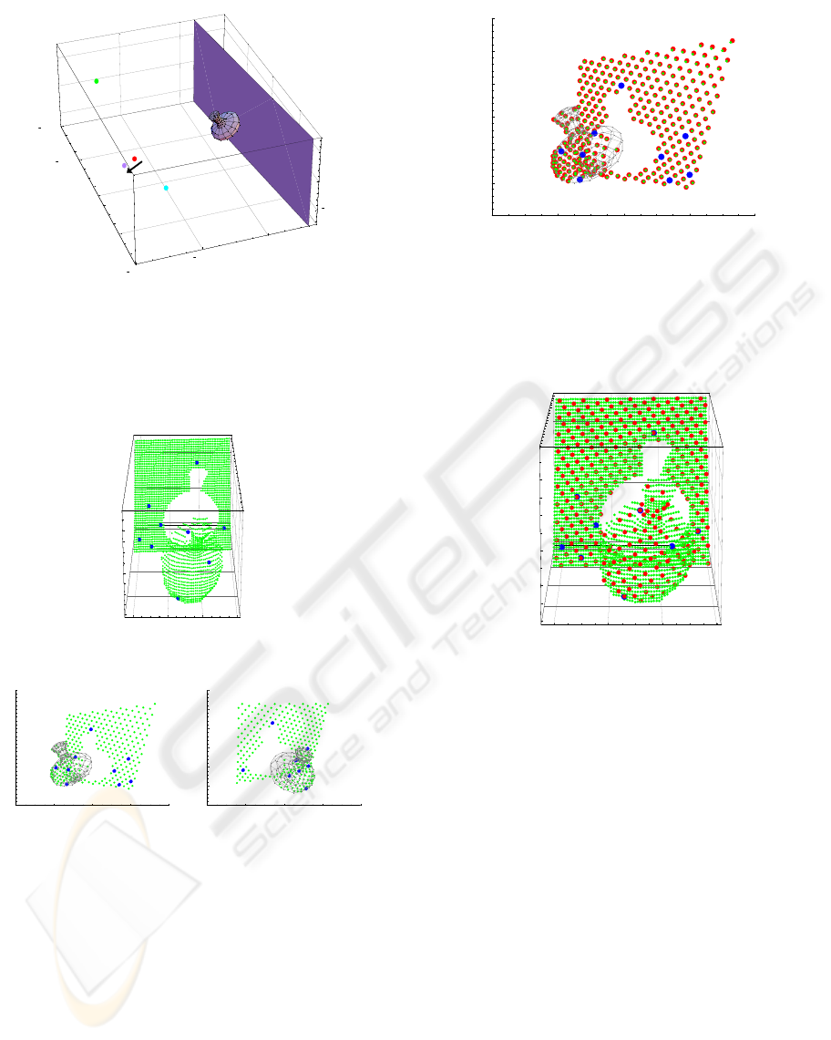
7.2 Moving 3D Range Sensor and 2D

Cameras

We next show the results from a moving 3D range

sensor and moving 2D cameras. As we have seen

in section 6, the multiple view geometry of moving

range sensors and moving 2D cameras can be de-

scribed by considering the projections from 4D space

to 3D space and 2D space. We translated the 3D range

sensor during the 3D measurement, and obtained the

3D data. C

and C

′

in Fig. 8 show the position of

the 3D range sensor before and after the translational

motion. C

and C

show 2 ﬁxed cameras. Fig. 9 (a)

MULTIPLE VIEW GEOMETRY FOR MIXED DIMENSIONAL CAMERAS

5000

15000

10000

5000

2500

5000

15000

10000

5000

15000

10000

5000

2500

5000

15000

10000

5000

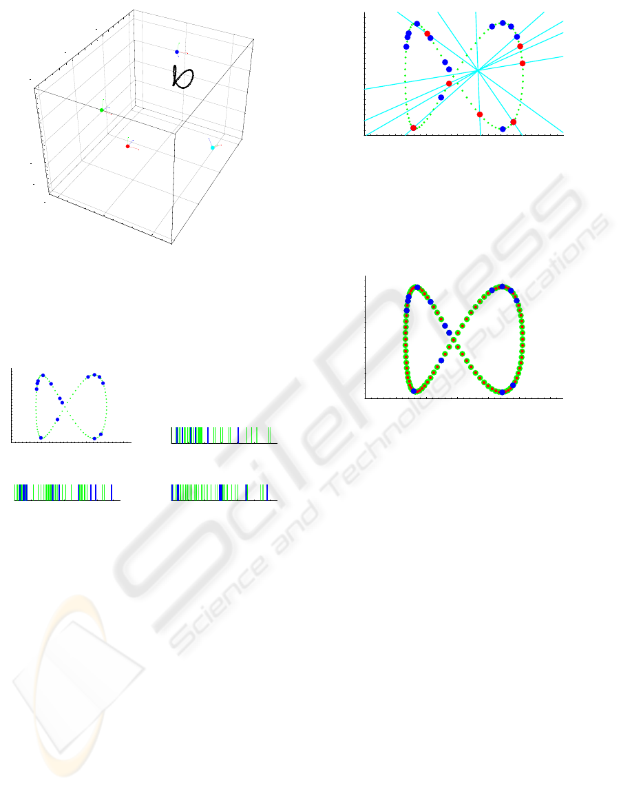
Figure 4: 3D scene. The black curve shows a locus of a

moving point X. The moving point X is observed by a 2D

camera, C

, and three 1D cameras, C

, C

and C

. The

three lines of each camera show the orientation of the cam-

era.

100 200 300 400 500 600

100

200

300

400

200 400 600 800 1000 1200

(a) (b)

200 400 600 800 1000 1200

Figure 5: The images of a 2D camera and three 1D cameras.

(a) shows the image of C

. (b), (c) and (d) show the image

of C

, C

and C

respectively. The green points and lines

in these images show the projection of a moving point. The

blue points and lines show corresponding basis points for

computing the multifocal tensors.

shows the 3D data measured by the translational 3D

range sensor. As we can see in this ﬁgure, the mea-

sured 3D data is distorted because of the motion of

the range sensor. The laser light of the range sensor

reﬂected at the surface of the object was observed by

2 cameras. The green points in Fig. 9 (b) and (c) show

the laser light observed in these 2 cameras. The blue

points in these data show basis corresponding points

used for computing the trifocal tensor. The extracted

trifocal tensor was used for transfering the 3D range

data into the image of camera C

. The green points

in Fig. 10 show the original image points and the red

points show the 3D data transfered by using the trifo-

100 200 300 400 500 600

100

200

300

400

Figure 6: The epipolar lines computed from the trifocal ten-

sor and the points in 1D line cameras. The blue points show

the basis points used for computing the trifocal tensor, and

the red points show some other corresponding points. Since

the epipolar lines go through the corresponding points, we

ﬁnd that the computed trifocal tensor is accurate.

100 200 300 400 500 600

100

200

300

400

Figure 7: The points in the 1D camera images are transfered

into the 2D camera image by using the extracted quadrifocal

tensor. The green points show the original loci in the image,

and the red points show the result of the point transfer.

cal tensor. As shown in this ﬁgure, the 3D data was

transfered properly by using the multiple view geom-

etry in 4D space, even if the range sensor moved dur-

ing the measurement.

We next computed the 3D range data from two

2D camera images and the extracted trifocal tensor.

Fig. 11 shows the points in the 3D image, which are

computed from the trifocal tensor. As shown in this

ﬁgure, the set of points in 2D camera images are trans-

fered into the points in the 3D range data properly by

using the proposed multiple view geometry. These

properties can be used for mapping the image textures

to the range image only by using point transfer.

8 CONCLUSIONS

In this paper, we showed that there exist multilinear

constraints on image coordinates, even if the dimen-

sions of camera images are different from each other.

We ﬁrst analyzed the multiple view geometry of gen-

eral mixed dimensional cameras. We next showed

VISAPP 2008 - International Conference on Computer Vision Theory and Applications

4000

2000

4000

2000

1000

2000

′

4000

2000

4000

2000

1000

2000

′

Figure 8: 3D scene. A 3D object (vase) is observed by a

moving 3D range sensor, C

, and two 2D cameras, C

, C

′

shows the position of the range sensor after a transla-

tional motion.

0200400600

200

400

3000

3500

4000

4500

(a)

200 400 600 800

100

200

300

400

500

600

200 400 600 800

100

200

300

400

500

600

(b) (c)

Figure 9: Range data and camera images. The green points

in (a) show the range data obtained from the range sensor,

and the green points in (b) and (c) show the laser points

observed in 2 cameras. The blue points in these images

show basis points used for computing the trifocal tensor.

the multilinear constraints of some example cases of

mixed dimensional cameras. The new multilinear

constraints can be used for describing the geometric

relationships between 1D line sensors, 2D cameras,

3D range sensors, etc. and thus they are useful for

calibrating sensor systems in which different types of

cameras and sensors are used together. The power of

200 400 600 800

100

200

300

400

500

600

Figure 10: The range data transfered into the camera image.

The green points show the original laser points observed

in the image, and the red points show the points transfered

from the 3D range data by using the trifocal tensor. The

blue points show the basis points used for computing the

trifocal tensor.

0200400600

200

400

3000

3500

4000

4500

Figure 11: The image data transfered into the range data.

The green points show the original laser points, and the red

points show the points transfered from the 2D camera im-

ages by using the trifocal tensor. The blue points show the

basis points used for computing the trifocal tensor.

the new multiple view geometry was shown by using

synthetic images in some mixed sensor systems.

REFERENCES

Faugeras, O. and Keriven, R. (1995). Scale-space and afﬁne

curvature. In Proc. Europe-China Workshop on Geo-

metrical Modelling and Invariants for Computer Vi-

sion, pages 17–24.

Faugeras, O. and Luong, Q. (2001). The Geometry of Mul-

tiple Images. MIT Press.

Hartley, R. and Schaffalitzky, F. (2004). Reconstruction

from projections using grassman tensors. In Proc. 8th

European Conference on Computer Vision, volume 1,

pages 363–375.

MULTIPLE VIEW GEOMETRY FOR MIXED DIMENSIONAL CAMERAS

Hartley, R. and Zisserman, A. (2000). Multiple View Geom-

etry in Computer Vision. Cambridge University Press.

Hayakawa, K. and Sato, J. (2006). Multiple View Geometry

in the Space-Time. In Proc. 7th Asian Conference on

Computer Vision, volume 2, pages 437–446.

Heyden, A. (1998). A common framework for multiple

view tensors. In Proc. 5th European Conference on

Computer Vision, volume 1, pages 3–19.

Shashua, A. and Wolf, L. (2000). Homography tensors: On

algebraic entities that represent three views of static or

moving planar points. In Proc. 6th European Confer-

ence on Computer Vision, volume 1, pages 507–521.

Sturm, P. (2002). Mixing catadioptric and perspective cam-

eras. In Proc. Workshop on Omnidirectional Vision.

Sturm, P. (2005). Multi-view geometry for general camera

models. In Proc. Conference on Computer Vision and

Pattern Recognition, pages 206–212.

Thirthala, S. and Pollefeys, M. (2005). Trifocal tensor for

heterogeneous cameras. In Proc. Workshop on Omni-

directional Vision.

Triggs, B. (1995). Matching constraints and the joint image.

In Proc. 5th International Conference on Computer

Vision, pages 338–343.

Wexler, L. and Shashua, A. (2000). On the synthesis of

dynamic scenes from reference views. In Proc. Con-

ference on Computer Vision and Pattern Recognition.

Wolf, L. and Shashua, A. (2001). On projection matrices

→ P

, k = 3, ··· , 6, and their applications in com-

puter vision. In Proc. 8th International Conference on

Computer Vision, volume 1, pages 412–419.

VISAPP 2008 - International Conference on Computer Vision Theory and Applications

REFERENCES

Faugeras, O. and Keriven, R. (1995). Scale-space and affine