
OPTICAL-FLOW FOR 3D ATMOSPHERIC MOTION ESTIMATION
Patrick H´eas and Etienne M´emin
INRIA -IRISA, Campus de Beaulieu, Rennes, France
Keywords:
3D Motion estimation, Variational methods, Optical-flow, Atmospheric dynamics, Physical-based model.
Abstract:
In this paper, we address the problem of estimating three-dimensional motions of a stratified atmosphere from
satellite image sequences. The complexity of three-dimensional atmospheric fluid flows associated to incom-
plete observation of atmospheric layers due to the sparsity of cloud systems makes very difficult the estimation
of dense atmospheric motion field from satellite images sequences. The recovery of the vertical component
of fluid motion from a monocular sequence of image observations is a very challenging problem for which no
solution exists in the literature. Based on a physically sound vertical decomposition of the atmosphere into
layers of different altitudes, we propose here a dense motion estimator dedicated to the extraction of three-
dimensional wind fields characterizing the dynamics of a layered atmosphere. Wind estimation is performed
over the complete three-dimensional space using a multi-layer model describing a stack of dynamic horizontal
layers of evolving thickness, interacting at their boundaries via vertical winds. The efficiency of our approach
is demonstrated on synthetic and real sequences.
1 INTRODUCTION
Geophysical motion characterization and analysis by
image sequence analysis is a crucial issue for nu-
merous scientific domains involved in the study of
climate change, weather forecasting, climate predic-
tion or biosphere analysis. The use of surface sta-
tion, balloon, and more recently in-flightaircraft mea-
surements and low resolution satellite images has im-
proved the estimation of wind fields and has been a
subsequent step for a better understanding of meteo-
rological phenomena. However, the network’s tempo-
ral and spatial resolutions may be insufficient for the
analysis of mesoscale dynamics. Recently, in an ef-
fort to avoid these limitations, another generation of
satellites sensors has been designed, providing image
sequences characterized by finer spatial and temporal
resolutions. Nevertheless, the analysis of motion re-
mains particularly challenging due to the complexity
of atmospheric dynamics at such scales.
Tools are needed to exploit this new generation
of satellite images and we believe that it is very im-
portant that the computer vision community gets in-
volved in such domain as they can potentially bring
relevant contributions with respect to the analysis of
spatio-temporal data.
Nevertheless in the context of geophysical mo-
tion analysis, standard techniques from Computer Vi-
sion, originally designed for bi-dimensional quasi-
rigid motions with stable salient features, appear to
be not well adapted (Horn and Schunck, 1981) (Leese
et al., 1971). The design of techniques dedicated to
fluid flow has been a step forward, towards the consti-
tution of reliable methodsto extract characteristic fea-
tures of flows (Anonymous)(Anonymous)(Zhouet al.,
2000). However, for geophysical applications, exist-
ing fluid-dedicated methods are all limited to horizon-
tal velocity estimation and neglect vertical motion.
All these methods are obviously not adapted to the
extraction of 3D measurements but also do not take
into account accurately luminance variations due to
3D motions. Such effects are occasionally important
at small scales and should be incorporated in the mo-
tion estimation method.
Geophysical flows are quite well described by ap-
propriate physical models. As a consequence in such
contexts, a physically-based approach can be very
powerful for analyzing incomplete and noisy image
data, in comparison to standard statistical methods.
The inclusion of physical a priori leads to novel ad-
vanced techniques for motion analysis or 3D informa-
tion recovery. This yields to new application domains
399
Héas P. and Mémin E. (2008).
OPTICAL-FLOW FOR 3D ATMOSPHERIC MOTION ESTIMATION.
In Proceedings of the Third International Conference on Computer Vision Theory and Applications, pages 399-406
DOI: 10.5220/0001071503990406
Copyright
c
SciTePress

impacting potentially studies of capital interest for our
everyday life, and obviously to the devise of proper
efficient techniques. This is thus a research domain
with wide perspectives. Our work is a contribution
towards this direction.
The method proposed in this paper is significantly
different from previous works on motion analysis by
satellite imagery. A main difference is that the data
model used in our method relies on an exact 3D phys-
ical model for pressure difference image observations
retrieved at different atmospheric levels. This inter-
acting layered model allows us to recover a vertical
motion information.
2 RELATED WORKS ON
OPTICAL FLOW
The problem of wind field recovery consists in esti-
mating the 3D atmospheric motion denoted by V(s,t)
from a 2D image sequence I(s,t), where (s,t) denote
the pixel and time coordinates. This problem is a
complex one, for which we have only access to pro-
jected information on cloudsposition and spectral sig-
natures provided by satellite observation channels. To
avoid the three-dimensional wind field reconstruction
problem, all developed methods have relied on the as-
sumption of negligible vertical winds and focused on
the estimation of a global apparent horizontal winds
related to top of clouds of different heights.
The estimation of the apparent motion v(s,t) as
perceived through image intensity variations (the so-
called optical-flow) relies principally on the tempo-
ral conservation of some invariants. The most com-
mon invariant used is the brightness constancy as-
sumption. This assumption leads to the well known
Optical-Flow Constraint (OFC) equation
v· ∇I(s,t) + I
t
(s,t) = 0 (1)
An important remark is that for image se-
quences showing evolving atmospheric phenomena,
the brightness consistency assumption does not allow
to model temporal distortions of luminance patterns
caused by 3D flow transportation. In spite of that,
most estimation methods used in the meteorology
community still rely on this crude assumption (Larsen
et al., 1998). In the case of transmittance imagery, the
Integrated Continuity Equation (ICE) provides a valid
invariant assumption for compressible flows (Fitz-
patrick, 1988) under the assumption that the temporal
derivatives of the integration boundaries compensate
the normal flows. This ICE model reads :
Z
ρdz
t
+ v.∇
Z
ρdz
+
Z
ρdz
divv = 0 (2)
where ρ and v denotethe fluid density and the den-
sity averaged horizontal motion field along the verti-
cal axis. Unlike the OFC, such models can compen-
sates mass departures observed in the image plan by
associating two-dimensional divergence to brightness
variations. But, for the case of satellite infra-red im-
agery, the assumption that I ∝
R
ρdz is flawed. More-
over, note that although the assumed boundary con-
dition is valid for incompressible flows, it is not real-
istic for compressible atmospheric flows observed at
a kilometer order scale. However, based on experi-
ments, authors proposed to apply directly this model
to the image observations (Anonymous) or to the in-
verse of the image intensities (Zhou et al., 2000).
Recently, under the assumption of negligible vertical
wind, the model of Eq. 2 has been applied to pres-
sure difference maps approximating the density inte-
grals (Anonymous).
The formulationsof Eq.1 and Eq.2 can not be used
alone, as they provide only one equation for two un-
knowns at each spatio-temporal locations (s,t), with
therefore a one dimensional family of solutions in
general. In order to remove this ambiguity and ro-
bustify the estimation, the most common assumption
consists to enforce a spatial local coherence. The lat-
ter can explicitly be expressed as a regularity prior in
a globalized smoothing scheme. Within this scheme,
spatial dependenciesare modeled on the complete im-
age domain and thus robustness to noise and low con-
trasted observations is enhanced. More precisely, the
motion estimation problem is defined as the global
minimization of an energy function composed of two
components :
J(v,I) = J
d
(v,I) +αJ
r
(v) (3)
The first component J
d
(v,I) called the data term,
expresses the constraint linking unknowns to obser-
vations while the second component J
r
(v), called the
regularization term, enforces the solution to follow
some smoothness properties. In the previous expres-
sion, α > 0 denotes a parameter controlling the bal-
ance between the smoothness and the globaladequacy
to the observation model. In this framework, Horn
and Schunck (Horn and Schunck, 1981) first intro-
duced a data term related to the OFC equation and
a first-order regularization of the two spatial compo-
nents u and v of velocity field v. In the case of trans-
mittance imagery of fluid flows, I =
R
ρdz, and using
the previously defined ICE model (Eq.2) leads to the
functional :
J
d
(v,I) =
Z
Ω
(I
t
(s) + v(s) · ∇I(s) + I(s)divv(s))
2
ds (4)
where Ω denotes the image domain.
Moreover, it can be demonstrated that a first order
VISAPP 2008 - International Conference on Computer Vision Theory and Applications
400

regularization is not adapted as it favors the estima-
tion of velocity fields with low divergence and low
vorticity. A second order regularization on the vortic-
ity and the divergence of the defined motion field can
advantageously be considered as proposed in (Anony-
mous)(Suter, 1994)(Anonymous) :
J
r
(v) =
Z
Ω
k ∇curlv(s) k
2
+ k ∇divv(s) k
2
ds (5)
Instead of relying on a L
2
norm, robust penalty
function φ
d
may be introduced in the data term for at-
tenuating the effect of observations deviating signifi-
cantly from the ICE constraint (Black and Anandan,
1996). Similarly, a robust penalty function φ
r
can be
used if one wants to handle implicitly the spatial dis-
continuities of the vorticity and divergence maps. In
the image plan, these discontinuities are nevertheless
difficult to relate to abrupt variations of clouds height.
Moreover, the robust approach does not allow points
of unconnectedregions, which belongto a same layer,
to interact during the motion estimation process.
3 MODELING A DYNAMICAL
STACK OF LAYERS
3.1 Integrated Continuity Equation for
3D Winds
Interesting models for 3D compressible atmospheric
motion observed through imagesequencesmay be de-
rived by integrating the 3D continuity equation ex-
pressed in the isobaric coordinate system (x, y, p). In
comparison to standard altimetric coordinates, iso-
baric coordinates are advantageous : they enable to
handle in a simple manner the compressibility of at-
mospheric flows while dealing directly with pressure
quantities, which will be used as observations in this
paper. In this coordinate system, the pressure function
p acts as a vertical coordinate. Let us denote the hori-
zontal wind components by v = (u,v) and the vertical
wind in isobaric coordinates by ω. The 3D continuity
equation reads (Holton, 1992) :
−
∂ω
∂p
=
∂u
∂x
+
∂v
∂y
p
(6)
By defining now two altimetric surfaces s
k
and s
k+1
with p(s
k
) > p(s
k+1
) related to a pressure difference
function δp
k
and a pressure-average horizontal wind
field v
k
δp
k
= p(s
k
) − p(s
k+1
)
v
k
=
1
δp
k
Z
p(s
k
)
p(s
k+1
)
vdp (7)
we have demonstrated in appendix I that the vertical
integration of Eq.6 in the altimetric interval [s
k
,s
k+1
]
yields under certain conditions to the following 3D-
ICE model:
gρ(s
k
)w(s
k
) − gρ(s
k+1
)w(s
k+1
) =
dδp
k
dt
+ δp
k
div(v
k
) (8)
where g and w denote thegravity constant and the ver-
tical wind in the standard altimetric coordinate sys-
tem (x,y,z). Note that this model appears to be a
generalization of the so called kinematic method ap-
plied in meteorology for the recovery of vertical mo-
tion (Holton, 1992). Indeed, by neglecting the first
term on the right hand side of Eq.8, vertical motion
can be expressed as :
w(s
k+1
) =
ρ(s
k
)w(s
k
)
ρ(s
k+1
)
−
δp
k
gρ(s
k+1
)
div(v
k
), (9)
which corresponds exactly to the kinematic estimate.
Note also that the ICE model (Eq.2) can be recov-
ered when vertical motion is neglected and for an at-
mosphere in hydrostatic equilibrium (δp = −g
R
ρdz).
On the right side of the 3D-ICE, vertical motion w
appears only on the integration boundaries, while
on the left side, pressure-average horizontal motion
v
k
appears within a standard optical flow expression
compensated by a divergence correcting term. Thus,
for pressure difference observations on layer bound-
aries, the 3D-ICE constitutes a possible 3D estimation
model.
3.2 Layer Decomposition
The layering of atmospheric flow in the troposphere
is valid in the limit of horizontal scales much greater
than the vertical scale height, thus roughly for hori-
zontal scales greater than 100 km. It is thus impossi-
ble to guarantee to truly characterize a layered atmo-
sphere with a local analysis performed in the vicin-
ity of a pixel characterizing a kilometer order scale.
Nevertheless, one can still decompose the 3D space
into elements of variable thickness, where only suffi-
ciently thin regions of such elements may really cor-
respond to common layers. Analysis based on such
a decomposition presents the main advantage of op-
erating at different atmospheric pressure ranges and
avoids the mix of heterogeneous observations.
Let us present the 3D space decompositionthat we
chose for the definition of the layers. The k-th layer
corresponds to the volume lying in between an upper
surface s
k+1
and a lower surface s
k
. These surfaces
s
j
are defined by the height of top of clouds belong-
ing to the j-th layer. They are thus defined only in
areas where there exists clouds belonging to the j-th
OPTICAL-FLOWFOR 3D ATMOSPHERIC MOTION ESTIMATION
401
layer, and remains undefined elsewhere. The mem-
bership of top of clouds to the different layers is de-
termined by cloud classification maps. Such classifi-
cations which are based on thresholds of top of cloud
pressure, are routinely provided by the EUMETSAT
consortium, the European agency which supplies the
METEOSAT satellite data.
3.3 Sparse Pressure Difference
Observations
Top of cloud pressure images are also routinely pro-
vided by the EUMETSAT consortium. They are de-
rived from a radiative transfer model using ancil-
lary data obtained by analysis or short term fore-
casts (Lutz, 1999).
We denote by C
k
the class corresponding to the k-
th layer. Note that the top of cloud pressure image de-
noted by p
S
is composed of segments of top of cloud
pressure functions p(s
k+1
) related to the different lay-
ers. That is to say : p
S
= {
S
k
p(s
k+1
,s); s ∈ C
k
}. Thus,
pressure images of top of clouds are used to consti-
tute sparse pressure maps of the layer upper bound-
aries p(s
k+1
). As in satellite images, clouds lower
boundaries are always occluded, we coarsely approx-
imate the missing pressure observations p(s
k
) by an
average pressure value p
k
observed on top of clouds
of the layer underneath. Finally, for the k-th layer, we
define observations h
k
as pressure differences :
p
k
− p
S
= h
k
= δp
k
(s) if s ∈ C
k
6= δp
k
(s) if s ∈
¯
C
k
,
(10)
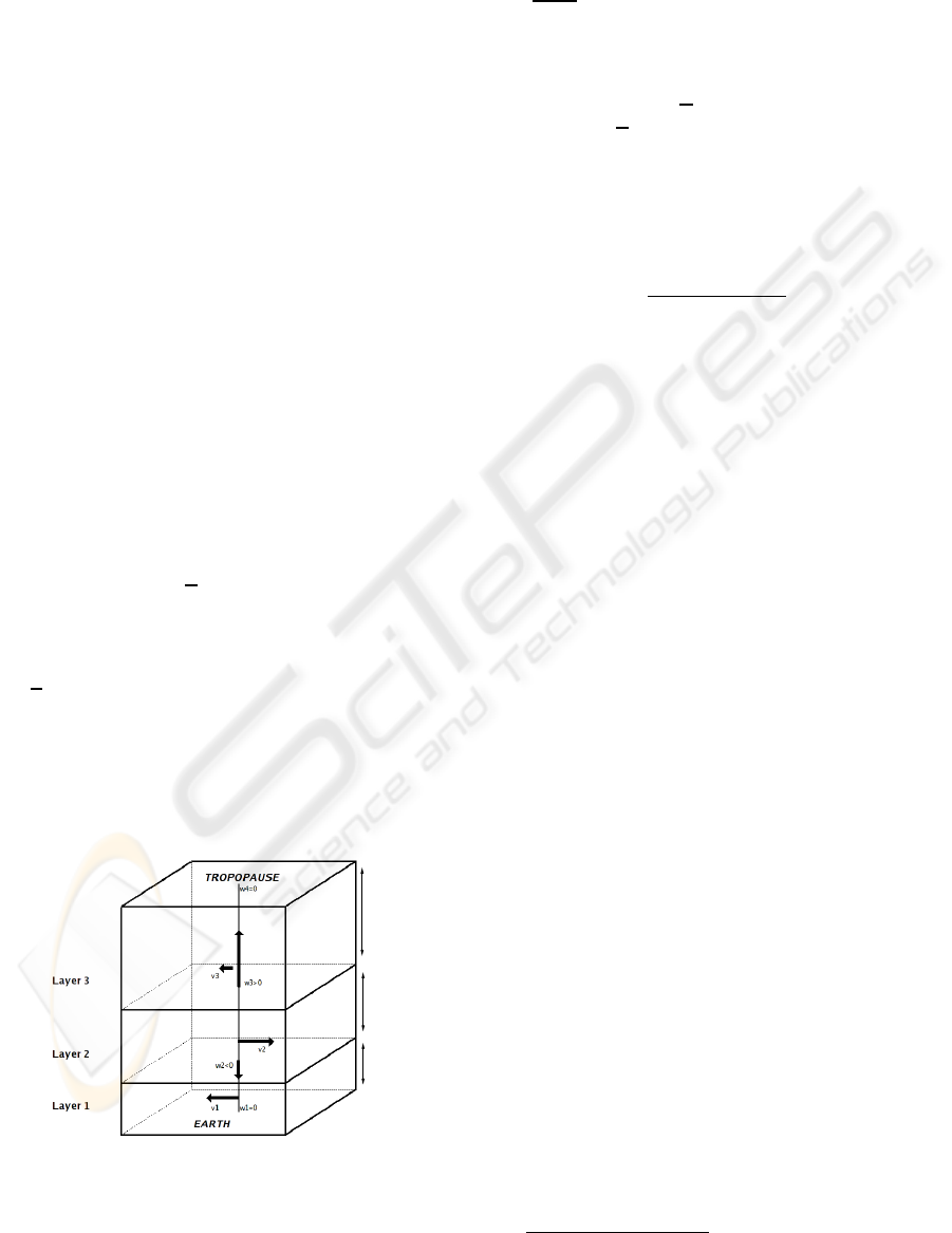
3.4 Layer Interacting Model
h2
h1
h3
Figure 1: Scheme of three interacting layers defined at a
given pixel location. The set of unknowns associated to the
corresponding 3D-ICE model is {v
1
,w
2
,v
2
,w
3
,v
3
}. For
the enhancement of the visual representation, pressure dif-
ference h
k
have been identified here to altimetric heights.
Eq.8 is thus valid for image observations h
k
re-
lated to the k-th layer on the spatial sub-domain C
k
:
d(h
k
)
dt
+ h
k
∇· v
k
= g(ρ
k
w
k
− ρ
k+1
w
k+1
) (11)
where for clarity we have simplified notations ρ(s
k
)
and w(s
k
) into ρ
k
and w
k
. Density maps ρ
k
are fixed
to a mean density value, which is computed according
to the mean pressures p
k
using the approximation :
ρ
k
≈ p
0
/(RT
0
)(p
k
/p
0
)
(γR)/g+1
, where p
0
, T
0
, γ and R
denote physical constants (Holton, 1992).
Integrating in time differential equation 11 along
the horizontal trajectories and applying the variation
of the constant tecnhique for the second member, we
obtain a time-integrated form :
˜
h
k
e
divv
k
− h
k
= g∆t
ρ
k
w
k
− ρ
k+1
w
k+1
divv
k
(e
divv
k
− 1) (12)
where the motion-compensatedimage h
k
(s+v
k
,t+∆t)
has been denoted for convenience by
˜
h
k
and where
∆t denotes the time interval expressed in seconds be-
tween two consecutive images.
For the lowest layer, the Earth boundary condition
implies : w
1
= 0. Let K denote the index of the high-
est layer. Another boundary conditions may be given
for the highest layer by the reasonable assumption
that vertical wind can be neglected at the tropopause
which acts like a cover : w
K+1
= 0. Thus, as the verti-
cal wind present on the upper bound of the k-th layer
is identical to the one present on the lower bound of
the (k + 1)-th layer, we have the following two sets of
unknowns : {v
k
: k ∈ [1,K]} and {w
k
: k ∈ [2,K]}. The
vertical wind unknowns act as variables materializing
horizontal wind interactions between adjacent layers.
Fig.1 schematizes an exampleof three interacting lay-
ers associated to a set of unknowns, according to the
3D-ICE model.
4 3D WIND ESTIMATION
4.1 Dedicated Robust Estimator
Since outside the class C
k
, h
k
defined in Eq.10 is not
relevant of the k-th layer, we introduce a masking op-
erator to removeunreliable observations by saturation
of a robust penalty function φ
d
. More explicitly, we
denote by I
C
k
the operator which is identity if pixel
belong to the class, and which returns a fixed value
out of the range taken by h
k
otherwise. Thus, apply-
ing this new masking operator in Eq.12, we obtain for
the k-th layer the robustdata term J
d
(v
k
,w
k
,w
k+1
,h
k
) =
Z
Ω
φ
d
˜
h
k
(s)exp{divv
k
(s)} − I
C
k
(h
k
(s))
+g∆t
ρ
k
w
k
(s) − ρ
k+1
w
k+1
(s)
divv
k
(s)
(1− exp{divv
k
(s)})
ds (13)
VISAPP 2008 - International Conference on Computer Vision Theory and Applications
402

A second order div-curl regularizer has been chosen
to constrain spatial smoothness of horizontal wind
fields. The latter was combined with a first order
regularizer enforcing regions of homogeneous verti-
cal winds. Note that we have restricted the regularizer
for vertical wind to be a first order one, as 3D diver-
gence and 3D vorticity vectors are inaccessible in a
layered model. The regularization term for the k-th
layer has been thus defined as J
r
(v
k
,w
k
) =
Z
Ω
α(k ∇curlv
k
(s) k
2
+k ∇divv
k
(s) k
2
)+βk ∇w
k
(s) k
2
ds, (14)
where β > 0 denotes a positive parameter. A Leclerc
M-estimator has been chosen for φ
d
for its advanta-
geous minimization properties (Holland and Welsch,
1977). The masking procedure together with the use
of this robust penalty function on the data term al-
lows discarding implicitly the erroneous observations
from the estimation process. It is important to outline
that, for the k-th layer, the method provides estimates
on all point s of the image domain Ω. Areas outside
the cloud classC
k
correspondto 3D interpolated wind
fields.
4.2 Large Horizontal Displacements
One major problem with the differential formula-
tion of Eq.11 is the estimation of large displace-
ments. However, on the opposite of the integrated
form of Eq.12 which is valid for high amplitude dis-
placements, this formulation presents the advantage
to be linear. A standard approach for tackling the
non-linear data term consists to apply successive lin-
earizations around a current estimate and to warp
a multiresolution representation of the data accord-
ingly. This approach relies on an image pyramid,
constructed by successive low-pass filtering and down
sampling of the original images. A large displace-
ment field
˜
v is first estimated at coarse resolution
where motion amplitude should be sufficiently re-
duced in order to make the initial differential data
model valid. Then, the estimation is refined through
an incremental fields v
′
while going down the pyra-
mid (Bergen et al., 1992). The latter are estimated
within a linear scheme by minimizing linearized
motion-compensated functionals : for the decompo-
sition v
k
=
˜
v + v
′
, Eq.13 is linearized around
˜
v and
yields to a motion-compensated linear formulation of
the data term. Let us denote by
˜
ζ
k
the coarse scale
divergence estimate div
˜
v and omit for sake of clarity
point coordinates s in the integrals. For the k-th layer,
the linearized data term reads J
d
(v
k
,w
k
,w
k+1
,h
k
) =
Z
Ω
φ
d
{e
˜
ζ
k
([
˜
h
k
∇
˜
ζ
k
+ ∇
˜
h
k
]
T
v
′
+
˜
h
k
) − I
C
k
(h
k
) (15)
+g∆t f(
˜
ζ
k
,w
k
,w
k+1
)}ds
where if
˜
ζ
k
6= 0, f(
˜
ζ
k
,w
k
,w
k+1
) =
ρ
k
w
k
− ρ
k+1
w
k+1
˜
ζ
k
1− e
˜
ζ
k
+ v
′
∇
˜
ζ
k
(
e
˜
ζ
k
− 1
˜
ζ
k
− e
˜
ζ
k
)
and if
˜
ζ
k
= 0, f(
˜
ζ
k
,w
k
,w
k+1
) = ρ
k+1
w
k+1
− ρ
k
w
k
4.3 Minimization Issues
In the proposed optimization scheme, we chose to
minimize a discretize version of functionals of Eq. 15
and Eq. 14. Let us denote by z
k
the robust weights
associated to the semi-quadratic penalty function re-
lated to the data term. Minimization is done by al-
ternatively solving large systems for unknowns v
k
,
w
k
and z
k
through a multigrid Gauss-Seidel solver.
More explicitly, all variables are first initialized to
zero. A global optimization procedure is then suc-
cessively operated at each level of the multiresolution
pyramid. This procedure first performs in a multigrid
optimization strategy, the minimization with respect
to v
k
of a linearized functional composed of the data
term defined in Eq.15 and of the second order smooth-
ness term defined in Eq.14. As variables {w
k
} and
{z
k
} are first frozen, this first step can be performed
independently for each layer level k ∈ [1, K]. Once
the minima have been reached, in a second step, fix-
ing variables {v
k
} and {z
k
}, the same functional is
minimized with respect to each w
k
,k ∈ [2,K].
Note that vertical wind w
k
is estimated consider-
ing variables related to the layer above the bound-
ary { w
k+1
,h
k
,
˜
h
k
,v
k
,z
k
} and the layer underneath the
boundary {w
k−1
,h
k−1
,
˜
h
k−1
,v
k−1
,z
k−1
}. Finally, in
a last step for each pixel locations and for each k ∈
[1,K], the robust weights z
k
are in turn updated while
variables {v
k
} and {w
k
} are kept fixed. The three pre-
vious minimization steps are iterated until a global
convergence criterion is reached, that is to say until
the variation of the estimated solution between two
consecutive iterations becomes sufficiently small.
It is important to point out that the proposed 3D
estimation methodology does not increase much the
complexity of the original non-linear horizontal mo-
tion estimation problem. Indeed, given horizontal
motion, the vertical wind estimation constitutes a lin-
ear quadraticproblemwhich can be efficiently solved.
5 EXPERIMENTAL EVALUATION
5.1 Synthetic Image Sequence
For an exhaustive evaluation,we have relied on a sim-
ulated flow of an atmosphere decomposed into K = 3
OPTICAL-FLOWFOR 3D ATMOSPHERIC MOTION ESTIMATION
403
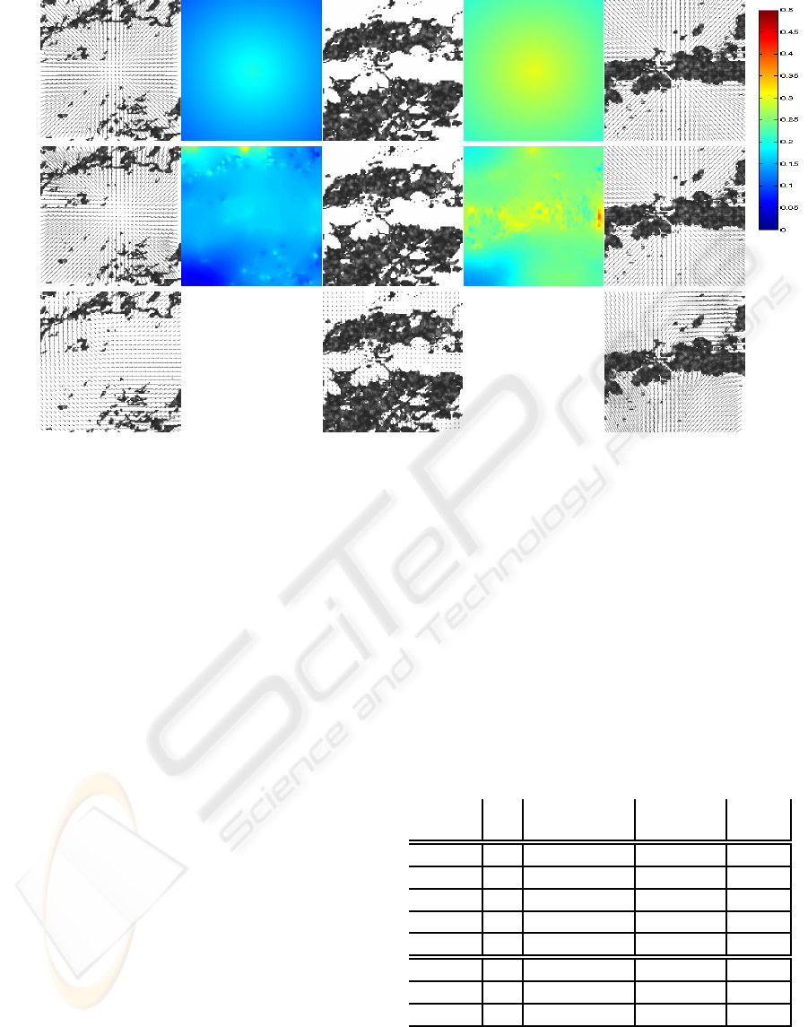
truth
3D-ICE
2D-ICE
v
1
w
2
v
2
w
3
v
3
Figure 2: Recovery of horizontal {v
1
,v
2
,v
3
} and vertical {w
2
,w
3
} wind fields. Simulated 3D winds (1
st
line). Horizontal
winds related to the high (left), the medium (middle) and the low (right) layer are superimposed on the cloud pressure
difference observations. Horizontal motion estimated with the 3D ICE model (2
nd
line) have been compared to results
obtained with a 2D version of the model (3
rd
line).
layers correspondingto low, medium and high clouds.
The resulting synthetic images have been chosen to
simulate a layered atmosphere contracting itself at
its basis, driven by ascendant winds, and expand-
ing itself at its top. Let us describe the 3D motion
simulation. A real cloud classification map (used in
the next experiment) has been employed to dissoci-
ate the layers, and to assign them to different image
regions C
k
. Thus, for each layers k, a sparse im-
age h
k
(t) of 128 by 128 pixels has been generated,
representative of cloud pressure difference measure-
ments on the assigned regions C
k
and of a fixed sat-
uration value on the complementary domain. A tex-
tured image of mean 600 hPa and with a standard de-
viation of 100 hPa has been used to simulate cloud
pressure difference values. The three resulting im-
ages are presented in figure 2. An horizontal mo-
tion v
1
issued from a divergent sink has been im-
posed to the lower layer, while on the middle layer
no horizontal winds v
2
= 0 has been considered. On
the higher layer, a motion v
3
issued from a divergent
source has been applied. The latter sink and source
possess a decreasing influence while going away from
the center of the image to its boundaries (motion am-
plitudes ranges in the interval ∼ 0 − 1.25 pixel per
frame, that is ∼ 0 − 4m.s
−1
). Non-uniform verti-
cal winds of strength w
2
∈ [0.1, 0.2]m.s
−1
and w
3
∈
[0.2,0.3]m.s
−1
have been simulated on the bound-
aries shared respectively by the lower and the medium
layers, and by the medium and the high layers re-
spectively. The latter horizontal and vertical winds
have been used to deform, according to the time in-
tegrated 3D-ICE model (Eq.12), image observations
[h
1
(t),h
2
(t),h
3
(t)] in order to generate propagated
images [h
1
(t+∆t),h
2
(t+∆t),h
3
(t+∆t)] with ∆t =900
seconds.
Barron’s error Speed bias RMSE
(degree) (pixel) (m/s)
3D-ICE w
3
0.027
w
2
0.028
v
3
6.426 0.099
v
2
0.138 0.002
v
1
3.566 0.058
2D-ICE v
3
29.608 0.210
v
2
6.331 0.112
v
1
38.276 0.161
Figure 3: Numerical evaluation. Barron angular error and
speed bias on horizontal winds {v
1
,v
2
,v
3
} and RMSE on
vertical wind {w
2
,w
3
} provided by the 3D-ICE model.
Comparison with horizontal winds produced by a 2D ver-
sion of the model.
VISAPP 2008 - International Conference on Computer Vision Theory and Applications
404
Horizontal and vertical winds which have been re-
trieved with the 3D estimator can be visualized in fig-
ure 2. For the three layer levels, vertical and horizon-
tal winds are accurately estimated in cloudy regions.
The estimator accuracy is evaluated in table 3, using
for horizontal wind the Barron angular error (Barron
et al., 1994) and the speed bias, and for vertical wind
the Root Mean Square Error (RMSE). In observations
free areas, vertical and horizontal winds appear to be
consistent with the divergent and ascendant motions.
Note that in the latter regions, the estimator acts as a
3D wind extrapolator. Moreover, it can be noticed that
the proposed layer interacting model increases signif-
icantly the estimation performances. In particular, the
convergent motion of the lower layer is well charac-
terized although only very few observations are avail-
able. For comparison purpose we have run on this
sequence the same estimator imposing a zero value to
the unknown vertical components. This comes to use
the 2D layered data model as proposed in (Anony-
mous). As a result, this estimator calculates indepen-
dent horizontal winds for the three different layers in
the very same numerical implementation setup as for
the 3D wind estimator. Results which are presented
in figure 2 and in table 3 show that the latter estimator
completely fails to accurately characterize horizon-
tal motion. This demonstrates that, although vertical
wind (∼ 0.1 − 0.3m.s.
−1
) is weak compared to hori-
zontal motion (∼ 0 − 4m.s.
−1
), its influence can not
be neglected in the estimation process. As evaluated
in table 3, a 3D data model clearly improves the re-
sults in such a situation.
5.2 Satellite Image Sequence
We then turned to qualitative evaluations on a
METEOSAT Second Generation meteorological se-
quence of 4 images acquired at a rate of an image
every 15 minutes, with a spatial resolution of 3 kilo-
meters at the center of the whole Earth image disk.
The images of 512 by 200 pixels cover an area over
the Gulf Guinea. The images are EUMETSAT top
of cloud pressure observations which are associated
to top of cloud classifications (Lutz, 1999). Accord-
ing to section 3.3, pressure images and classifications
maps have been used to derive pressure difference im-
age segments for 3 broad layers, at low, intermediate
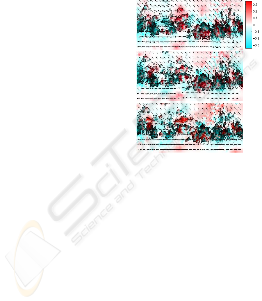
and high altitude. Figure 4 displays the pressure dif-
ference images related to the higher layer, together
with the 3D estimated wind fields. One can visual-
ize here large convective systems. They are charac-
terized by strong ascendant flows which are smoothly
reversed after bursting while reaching the tropopause
cover. Such scenarios have been correctly estimated
as shown in figure 4. Furthermore, let us remark that
the time-consistency and the correct range of wind
values estimated are a testimony of the stability of the
3D estimation method.
Figure 4: Estimation of 3D wind in atmospheric convective
systems. Cloud pressure difference images of the highest
layer at 3 consecutive times (from top to bottom). Estimated
horizontal wind vectors which have been plotted on the im-
ages range in the interval [0,10]m.s.
−1
. Retrieved verti-
cal wind maps on the highest layer lower boundary have
been superimposed on the pressure difference images with
a shaded red color for ascendant motion and a shaded blue
color for descendant motion. Vertical wind ranges in the
interval [−0.5,0.5]m.s.
−1
.
6 CONCLUSIONS
In this paper, we have presented a motion estimation
method solving for the first time the complex problem
of 3D winds field recovery from satellite image se-
quences. In order to manage incomplete observations,
physical knowledge on 3D mass exchanges between
atmospheric layers have been introduced within an
optical flow scheme.
The estimator is based on a functional minimiza-
tion. The data term relies on the 3D-ICE model which
describes the dynamics of an interacting stack of at-
mospheric layers. The 3D-ICE model applies on a
set of sparse pressure difference images related to the
different atmospheric layers. A method is proposed
OPTICAL-FLOWFOR 3D ATMOSPHERIC MOTION ESTIMATION
405

to reconstruct such observations from satellite top of
cloud pressure images and classification maps. To
overcome the problem of sparse observations, a ro-
bust estimator is introduced in the data term. The
data term is combined to a regularizers preserving bi-
dimensional divergent and vorticity structures of the
three-dimensional flow and enforcing regions of ho-
mogeneous vertical winds.
An evaluationfirst performedon a synthetic image
sequence, and latter on a METEOSAT pressure image
sequences demonstrate the stability and the efficiency
of the method even in the difficult case of very sparse
image observations.
REFERENCES
Barron, J., Fleet, D., and Beauchemin, S. (1994). Perfor-
mance of optical flow techniques. Int. J. Computer
Vision, 12(1):43–77.
Bergen, J., Burt, P., Hingorani, R., and Peleg, S. (1992). A
three-frame algorithm for estimating two-component
image motion. IEEE Trans. Pattern Anal. Machine
Intell., 14(9):886–895.
Black, M. and Anandan, P. (1996). The robust estimation of
multiple motions: Parametric and piecewise-smooth
flow fields. Computer Vision and Image Understand-
ing, 63(1):75–104.
Fitzpatrick, J. (1988). The existence of geometrical
density-image transformations corresponding to ob-
ject motion. Comput. Vision, Graphics, Image Proc.,
44(2):155–174.
Holland, P. and Welsch, R. (1977). Robust regression using
iteratively reweighted least-squares. Commun. Statis.-
Theor. Meth., A6(9):813–827.
Holton, J. (1992). An introduction to dynamic meteorology.
Academic press.
Horn, B. and Schunck, B. (1981). Determining optical flow.
Artificial Intelligence, 17:185–203.
Larsen, R., Conradsen, K., and Ersboll, B. (1998). Estima-
tion of dense image flow fields in fluids. IEEE trans.
on Geoscience and Remote sensing, 36(1):256–264.
Leese, J., Novack, C., and Clark, B. (1971). An automated
technique for obtained cloud motion from geosyn-
chronous satellite data using cross correlation. Jour-
nal of applied meteorology, 10:118–132.
Lutz, H. (1999). Cloud processing for meteosat second
generation. Technical report, European Organisation
for the Exploitation of Meteorological Satellites (EU-
METSAT), Available at : http://www.eumetsat.de.
Suter, D. (1994). Motion estimation and vector splines. In
Proc. Conf. Comp. Vision Pattern Rec., pages 939–
942, Seattle, USA.
Zhou, L., Kambhamettu, C., and Goldgof, D. (2000). Fluid
structure and motion analysis from multi-spectrum 2d
cloud images sequences. In Proc. Conf. Comp. Vision
Pattern Rec., volume 2, pages 744–751, USA.
APPENDIX I
Vertical Integration of the Continuity
Equation
For compressible fluids, the continuity equation in the
(x,y, p) coordinates system reads:
−
∂ω
∂p
=
∂u
∂x
+
∂v
∂y
p
(16)
Let us denote by s
k
and s
k+1
altimetric surfaces with
p(s
k
) > p(s
k+1
). According to the Leibnitz for-
mula, integrating Eq.16 in the varying pressure inter-
val [p(s
k+1
), p(s
k
)] yields to :
[ω]
s
k+1
s
k
= div
p
Z
p(s
k
)
p(s
k+1
)
vdp− v(s
k
).∇
xy
(p(s
k
)
s
k
+ v(s
k+1
).∇
xy
(p(s
k+1
))
s
k+1
(17)
Moreover, expandingω in the (x, y, z) coordinates sys-
tem and using the hydrostatic assumption (
∂p
∂z
= −ρg)
yields to
ω =
dp
dt
=
∂p
∂t
+ v· ∇
xy
(p)− wρg, (18)
where w is the vertical velocity in z coordinates and
where we have introduced the density functions ρ and
the gravity constant g. Assuming that the surface s
k
is
flat in the vicinity of a pixel, by merging Eq. 17 and
Eq. 18, we obtain
g[ρw]
s
k
s
k+1
+
∂(p(s
k+1
) − p(s
k
))
∂t
I
s
≃ div
p
Z
p(s
k
)
p(s
k+1
)
vdp (19)
where we have denoted by I
s
the altimetric interval
between surfaces s
k
and s
k+1
. Let us now define the
following quantities :
δp
k
= p(s
k
) − p(s
k+1
)
v
k
=
1
δp
k
Z
p(s
k
)
p(s
k+1
)
vdp (20)
Considering the reasonable approximation
div(v
k
)
p
≃ div(v
k
)
I
s
, we can then rewrite Eq. 19 as
gρ(s
k
)w(s
k
) − gρ(s
k+1
)w(s
k+1
) ≃
∂δp
k
∂t
I
s
+ v
k
· ∇
xy
(δp
k
)
I
s
+ δp
k
div(v
k
)
I
s
(21)
Simplifying notations of operators defined for the al-
timetric interval I
s
, we obtain the relation :
gρ(s
k
)w(s
k
) − gρ(s
k+1
)w(s
k+1
) ≃
dδp
k
dt
+ δp
k
div(v
k
), (22)
which consitutes a proper image-adapted model for
observations δp
k
related to a layer defined in the in-
terval I
s
.
VISAPP 2008 - International Conference on Computer Vision Theory and Applications
406
