
MULTI-CHANNEL BIOSIGNAL ANALYSIS FOR AUTOMATIC
EMOTION RECOGNITION
Jonghwa Kim and Elisabeth Andr´e
Institute of Computer Science, University of Augsburg, Eichleitnerstr. 30, D-86159 Augsburg, Germany
Keywords:
Biosignal, emotion recognition, physiological measures, skin conductance, electrocardiogram, electromyo-
gram, respiration, affective computing, human-computer interaction, musical emotion, autonomic nervous
system, arousal, valence, feature extraction, pattern recognition.
Abstract:
This paper investigates the potential of physiological signals as a reliable channel for automatic recognition
of user’s emotial state. For the emotion recognition, little attention has been paid so far to physiological
signals compared to audio-visual emotion channels such as facial expression or speech. All essential stages
of automatic recognition system using biosignals are discussed, from recording physiological dataset up to
feature-based multiclass classification. Four-channel biosensors are used to measure electromyogram, electro-
cardiogram, skin conductivity and respiration changes. A wide range of physiological features from various
analysis domains, including time/frequency, entropy, geometric analysis, subband spectra, multiscale entropy,
etc., is proposed in order to search the best emotion-relevant features and to correlate them with emotional
states. The best features extracted are specified in detail and their effectiveness is proven by emotion recogni-
tion results.
1 INTRODUCTION
In human communication, expression and under-
standing of emotions facilitate to complete the mutual
sympathy. To approach it in human-machine interac-
tion, we need to equip machines with the means to
interpret and understand human emotions without in-
put of user’s translated intention. Hence, one of the
most important prerequisites to realize such an ad-
vanced user interface is a reliable emotion recogni-
tion system which guarantees acceptable recognition
accuracy, robustness against any artifacts, and adapt-
ability to practical applications. It is about to model,
analyze, process, train, and classify emotional fea-
tures measured from the implicit emotion channels of
human communication, such as speech, facial expres-
sion, gesture, pose, physiological responses, etc. In
this paper we concentrate on finding emotional cues
from various physiological measures.
Recently many works on engineering approaches
to automatic emotion recognition have been reported.
For an overview we refer to (Cowie et al., 2001). Par-
ticularly, most efforts have been taken to recognize
human emotions using audiovisual channels of emo-
tion expression, facial expression, speech, and ges-
ture. Relatively little attention, however, has been
paid so far to using physiological measures. Rea-
sons are some significant limitations resulting from
the use of physiological signals for emotion recogni-
tion. The main difficulty lies in the fact that it is a
very hard task to uniquely map subtle physiological
patterns onto specific emotional states. As an emo-
tion is a function of time, context, space, culture, and
person, physiological patterns may also widely differ
from user to user and from situation to situation.
In this paper, we treat all essential stages of auto-
matic emotion recognition system using physiological
measures, from data collection up to classification of
four typical emotions (joy, anger, sadness, pleasure)
using four-channel biosignals. The work in this pa-
per is novel in trying to recognize naturally induced
musical emotions using physiological changes, in ac-
quiring the physiological dataset through everyday
life recording over many weeks from multiple sub-
jects, in finding emotion-relevant ANS (autonomic
nervous system) specificity through various feature
contents, and in designing an emotion-specific classi-
fication method. After the calculation of a great num-
ber of features (a total of 110 features) from various
feature domains, we try to identify emotion-relevant
features using the backward feature selection method
combined with a linear classifier. These features can
be directly used to design affective human-machine
interfaces for practical applications.
124
Kim J. and André E. (2008).
MULTI-CHANNEL BIOSIGNAL ANALYSIS FOR AUTOMATIC EMOTION RECOGNITION.
In Proceedings of the First International Conference on Bio-inspired Systems and Signal Processing, pages 124-131
DOI: 10.5220/0001063301240131
Copyright
c
SciTePress

2 RELATED RESEARCH
A significant amount of work has been conducted by
Picard and colleagues at MIT Lab who showed that
certain affective states may be recognized by using
physiological data including heart rate, skin conduc-
tivity, temperature, muscle activity and respiration ve-
locity (Healey and Picard, 1998). They used person-
alized imagery to elicit target emotions from a sin-
gle subject who had two years’ experience in act-
ing, and achieved overall 81% recognition accuracy
in eight emotions by using hybrid linear discrimi-
nant classification (Picard et al., 2001). Nasoz et
al. (Nasoz et al., 2003) used movie clips based on
the study by Gross and Levenson (Gross and Leven-
son, 1995) for eliciting target emotions from 29 sub-
jects and achieved best emotion classification accu-
racy of 83% through the Marquardt Backpropagation
algorithm (MBP). More recently, interesting user-
independent emotion recognition system is reported
by Kim et al. (Kim et al., 2004). They developed
a set of recording protocols using multimodal stimuli
(audio, visual, and cognitive) to evoke targeted emo-
tions (sadness, stress, anger, and surprise) from the
175 children aged from five to eight years. Classi-
fication ratio of 78.43% for three emotions (sadness,
stress, and anger) and 61.76% for four emotions (sad-
ness, stress, anger, and surprise) has been achieved by
adopting support vector machine as pattern classifier.
Note that the recognition rates in the privious
works should be strongly dependent on the datasets
they used and context of subjects. Moreover, the
physiological datasets used in most of the previous
works are gathered by using visual elicitation mate-
rials in a lab setting. The subjects then “tried and
felt” or “acted out” the target emotions while look-
ing at selected photos or watching movie clips that
are carefully prearranged to the emotions. It means,
extremely speaking, that the recognition results were
achieved for specific users in specific contexts with
the “forced” emotional states.
3 MUSICAL EMOTION
INDUCTION
A well established mechanism of emotion induction
would be either to imagine or to recall from individ-
ual memory. Emotional reaction can be triggered by
a specific cue and be evoked by an experimental in-
struction to imagine certain events. On the other hand,
it can spontaneously be resurged in memory. Mu-
sic is a pervasive element accompanying many highly
significant events in human social life and particular
pieces of music are often connected to significant per-
sonal memories. This claims that certain music can
be a powerful cue in bringing emotional experiences
from memory back into awareness. Since music lis-
tening is often done by an individual in isolation, the
possible artifacts by social masking and social inter-
action may be minimized in the experiment. Further-
more, like odors, music may be treated at lower lev-
els of the brain that are particularly resistant to mod-
ifications by later input, contrary to cortically based
episodic memory (LeDoux, 1992).
anger
joy
sadness
pleasure
high arousal
low arousal
negative
positive
energetic
calm
anxious
happy
major
simple
complex
(song1)
(song2)
(song3)
(song4)
minor
fast
slow
soft
laud
high pitch
staccato
legato
low pitch
Figure 1: Reference emotional cues in music based on
the 2D emotion model. Metaphoric cues for song selec-
tion: song1 (enjoyable, harmonic, dynamic, moving), song2
(noisy, loud, irritating, discord), song3 (melancholic, sad
memory), song4 (blissful, pleasurable, slumberous, tender).
To collect a database of physiological signals in
which the targeted emotions (joy, anger, sadness,
pleasure)
1
can be naturally reflected without any de-
liberate expression, we decided to use musical induc-
tion method, recording physiological signals while
the subjects are listening to different music songs.
The subjects were three males (two students and an
academic employee) between 25-38 years old and
enjoyed listening to music everyday. The subjects
individually handpicked four music songs by them-
selves that should spontaneously evoke their emo-
tional memories and certain moods corresponding to
the four target emotions. Figure 1 shows the mu-
sical emotion model referred to for the selection of
their songs. Generally, emotional responses to music
would vary greatly from individual to individual de-
pending on their unique past experiences. Moreover,
1
We note that these four expression words are used to
cover each quadrant in the 2D emotion model, i.e. joy
should represent all emotions with high arousal and positive
valence, anger with high arousal and negative, sadness with
low arousal and negative, and pleasure with low arousal and
positive valence.
MULTI-CHANNEL BIOSIGNAL ANALYSIS FOR AUTOMATIC EMOTION RECOGNITION
125
cross-cultural comparisons in literature suggest that
the emotional responses can be quite differentially
emphasized by different musical cultures and train-
ing. This is why we advised the subjects to choose
themselves the songs that recall their individual spe-
cial memories with respect to the target emotions.
For the experiment, we prepared a quiet listening
room in our institute in order to ensure the subjects
to unaffectedly feel the emotions from the music. For
the recording, the subject needs to position himself
the sensors by instruction posters in the room, to ap-
ply the headphones, and to select a song from his song
list saved in the computer. When he does mouse-click
just at the start of recording, the recording and music
systems are automatically setting up by preset values
for each song. Recording schedule was determined
by the subjects themselves too, at any time when they
will listen to music and which song they choose. It
means, different from methods used in other studies,
that the subjects were not forced to participate in a
lab setting scenario and to use prespecified stimula-
tion materials. We believe that this voluntary partic-
ipation of the subjects during our experiment might
be a help to obtain a high-quality dataset with natural
emotions. The physiological signals are acquired us-
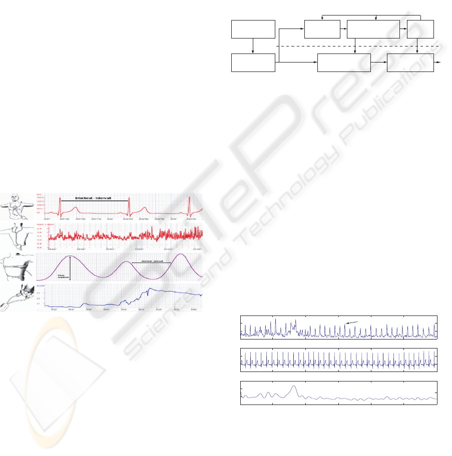
Position Typical Waveform
(a)
(b)
(c)
(d)
Figure 2: Position and typical waveforms of the biosensors:
(a) ECG, (b) EMG, (c) RSP, (d) SC.
ing the Procomp Infiniti
TM
(www.mindmedia.nl) with
four biosensors, electromyogram (EMG), skin con-
ductivity (SC), electrocardiogram (ECG), and respi-
ration (RSP). The sampling rates are 32 Hz for EMG,
SC, and RSP, and 256 Hz for ECG. The positions
and typical waveforms of the biosensors we used
are illustrated in Fig. 2. We used pre-gelled single
Ag/AgCl electrodes for ECG and EMG sensors and
standard single Ag/AgCl electrodes fixed with two
finger bands for SC sensor. A stretch sensor using
latex rubber band fixed with velcro respiration belt is
used to capture breathing activity of the subjects. It
can be worn either thoracically or abdominally, over
clothing.
During the three months, a total of 360 samples
(90 samples for each emotion) from three subjects is
collected. Signal length of each sample is between
3-5 minutes depending on the duration of the songs.
4 METHODOLOGY
Overall structure of our recognition system is illus-
trated in Figure 3.
Preprocessing
(Segment, Denoise,
Filtering etc.)
Feature
Calculation
(# < 110)
Multiclass
Classification
(pLDA, MDC)
Feature
Calculation
(110 Features)
Feature
Selection/Reduction
(# < 110)
Learning
4-channel
Biosignals
(ECG,EMG,SC,RSP)
Test Patterns
Training
Patterns
Training
Classification
Figure 3: Block diagram of supervised statistical classifica-
tion system for emotion recognition.
4.1 Preprocessing
Different types of artifacts were observed in all the
four channel signals, such as transient noise due
to movement of the subjects during the recording,
mostly at the begin and end of the each recording.
Thus, uniformly for all subjects and channels, we seg-
mented the signals into final samples with fixed length
of 160 seconds by cutting out from the middle part
of each signal. Particularly to the EMG signal, we
needed to pay closer attention because the signal con-
tains artifacts generated by respiration and heart beat
(Fig. 4). It was due to the position of EMG sensor at
the nape of the neck. For other signals we used per-
tinent lowpass filters to remove the artifacts without
loss of information.
0
10 20 30 sec
10 20 30 sec
10 20 30 sec
0
0
2
4
6
8
2
4
6
8
-1K
0
1K
2K
(a) EMG raw
(b) Corresponding ECG raw
(c) EMG filtered
heart beat artefacts
µVµVµV
Figure 4: Example of EMG signal with heart beat artifacts
and denoised signal.
4.2 Measured Features
From the four channel signals we calculated a total of
110 features from various analysis domains includ-
ing conventional statistics in time series, frequency
BIOSIGNALS 2008 - International Conference on Bio-inspired Systems and Signal Processing
126

domain, geometric analysis, multiscale sample en-
tropy, subband spectra, etc. For the signals with non-
periodic characteristics, such as EMG and SC, we fo-
cused on capturing the amplitude variance and local-
izing the occurrences (number of transient changes)
in the signals.
4.2.1 Electrocardiogram (ECG)
To obtain subband spectrum of the ECG signal we
used the typical 1024 points fast Fourier transform
(FFT) and partitioned the coefficients within the fre-
quency range 0-10 Hz into eight non-overlappingsub-
bands with equal bandwidth. First, as features, power
mean values of each subband and fundamental fre-
quency (F0) are calculated by finding maximum mag-
nitude in the spectrum within the range 0-3 Hz. To
capture peaks and their locations in subbands, sub-
band spectral entropy(SSE) is computed for each sub-
band. To compute the SSE, it is necessary to convert
each spectrum into a probability mass function (PMF)
like form. Eq. 1 is used for the normalization of the
spectrum.
x
i
=
X
i
∑
N
i=1
X
i
, for i = 1...N (1)
where X
i
is the energy of i
t
h frequency component of
the spectrum and
˜
x = {x
1
... x
N
} is to be considered
as the PMF of the spectrum. In each subband the SSE
is computed from
˜
x by
H
sub
= −
N
∑
i=1
x
i
· log
2
x
i
(2)
By packing the eight subbands into two bands, i.e.,
subbands 1-3 as low frequency (LF) band and sub-
bands 4-8 as high frequency (HF) band, the ratios of
LF/HF bands are calculated from the power mean val-
ues and the SSEs.
To obtain the HRV (heart rate variability) from
the continuous ECG signal, each QRS complex is de-
tected and the RR intervals (all intervals between ad-
jacent R waves) or the normal-to-normal (NN) inter-
vals (all intervals between adjacent QRS complexes
resulting from sinus node depolarization) are deter-
mined. We used the QRS detection algorithm of Pan
and Tompkins (Pan and Tompkins, 1985) in order to
obtain the HRV time series. Figure 5 shows example
of R wave detection and interpolated HRV time series,
referring to the increases and decreases over time in
the NN intervals.
In time-domain of the HRV, we calculated statis-
tical features including mean value, standard devia-
tion of all NN intervals (SDNN), standard deviation
of first difference of the HRV, the number of pairs
0
500 1000 1500 2000 2500
sample
sample
sample
0
500 1000 1500 2000 2500
0
500 1000 1500 2000 2500
0
2K
-2K
0
2K
-2K
0
2K
-2K
0
2
4 6 8 10
sec
sec
0.65
0.7
RR Interval_n
RR Interval_n+1
SD2
SD1
SD1 = 4.7 ms
SD2 = 15.8 ms
(b)
(c)
(a) (d)
(e)
µVµVµV
Figure 5: Example of ECG Analysis: (a) raw ECG sig-
nal with respiration artifacts, (b) detrended signal, (c) de-
tected RR interbeats, (d) interpolated HRV time series, (e)
Poincar´e plot of the HRV time series.
of successive NN intervals differing by greater than
50 ms (NN50), the proportion derived by dividing
NN50 by the total number of NN intervals. By cal-
culating the standard deviations in different distances
of RR interbeats, we also added Poincar´e geometry
in the feature set to capture the nature of interbeat
(RR) interval fluctuations. Poincar´e plot geometry is
a graph of each RR interval plotted against the next
interval and provides quantitative information of the
heart activity by calculating the standard deviations
of the distances of the R − R(i) to the lines y = x and
y = −x + 2∗ R− R
m
, where R− R
m
is the mean of all
R− R(i), (Kamen et al., 1996). Figure 5.(e) shows an
example plot of the Poincar´e geometry. The standard
deviations SD
1
and SD
2
refer to the fast beat-to-beat
variability and longer-term variability of R − R(i) re-
spectively.
Entropy-based features from the HRV time se-
ries are also considered. Based on the so-called ap-
proximate entropy and sample entropy proposed in
(Richmann and Moorman, 2000), a multiscale sam-
ple entropy (MSE) has been introduced (Costa et al.,
2005) and successfully applied to physiological data,
especially for analysis of short and noisy biosig-
nal. Given a time series {X
i
} = {x
1
,x
2
,...,x
N
} of
length N, the number (n
(m)
i
) of similar m-dimensional
vectors y
(m)
( j) for each sequence vectors y
(m)
(i) =
{x
i
,x
i+1
,...,x
i+m−1
} is determined by measuring their
respective distances. The relative frequency to find
the vector y
(m)
( j) within a tolerance level δ is defined
by
C
(m)
i
(δ) =
n
(m)
i
N − m + 1
(3)
The approximate entropy, h
A
(δ,m), and the sample
entropy, h
S
(δ,m) are defined as
MULTI-CHANNEL BIOSIGNAL ANALYSIS FOR AUTOMATIC EMOTION RECOGNITION
127
h
A
(δ,m) = lim
N→∞
[H
(m]
N
(δ) − H
(m+1)
N
(δ)], (4)
h
S
(δ,m) = lim
N→∞
−ln
C
(m+1)
(δ)
C
(m)
(δ)
, (5)
where
H
(m)
N
(δ) =
1
N − m + 1
N−m+1
∑
i=1
lnC
(m)
i
(δ), (6)
Because of advantage of being less dependent on time
series length N, we applied the sample entropy h
S
to coarse-grained versions (y
(τ)
j
) of the original HRV
time series {X
i
},
y
j
(τ) =
1
τ
jτ
∑
i=( j−1)τ+1
x
i
, 1 ≤ j ≤ N/τ, τ = 1,2, 3,...
(7)
The time series {X
i
} is first divided into N/τ seg-
ments by non-overlapped windowing with length of
scale factor τ and then the mean value of each seg-
ment is calculated. Note that for scale one y
j
(1) = x
j
.
From the scaled time series y
j
(τ) we obtain the m-
dimensional sequence vectors y
(m)
(i,τ). Finally, we
calculate the sample entropy h
S
for each sequence
vector y
j
(τ). In our analysis we used m = 2 and fixed
δ = 0.2σ for all scales, where σ is the standard de-
viation of the original time series x
i
. Note that using
the fixed tolerance level δ as a percentage of the stan-
dard deviation corresponds to initial normalizing of
the time series and it thus enables that h
S
does not de-
pend on the variance of the original time series, but
only on their sequential ordering.
In frequency-domainof the HRV time series, three
frequency bands are of interest in general; very-
low frequency (VLF) band (0.003-0.04 Hz), low fre-
quency (LF) band (0.04-0.15 Hz), and high frequency
(HF) band (0.15-0.4 Hz). From these subband spec-
tra, we computed dominant frequency and power of
each band by integrating the power spectral densi-
ties (PSD) obtained by using Welch’s algorithm, and
ratio of power within the low-frequency and high-
frequency band (LF/HF). Since the parasympathetic
activity dominates at high frequency, the ratio of
LF/HF is generally thought to distinguish sympathetic
effects from parasympathetic effects(Malliani, 1999).
4.2.2 Respiration (RSP)
Including the typical statistics of the raw RSP signal
we calculated similar types of features like the ECG
features, power mean values of three subbands (ob-
tained by dividing the Fourier coefficients within the
range 0-0.8 Hz into non-overlapped three subbands
with equal bandwidth), and the set of subband spec-
tral entropies (SSE).
In order to investigate inherent correlation be-
tween respiration rate and heart rate, we considered
a novel feature content for the RSP signal. Since
RSP signal exhibits quasi periodic waveform with si-
nusoidal property, it is not unreasonable to process
HRV like analysis for the RSP signal, i.e. to esti-
mate breathing rate variability (BRV). After detrend-
ing with mean value of the entire signal and low-
pass filtering, we calculated the BRV by detecting the
peaks in the signal using the maxima ranks within
each zero-crossing. From the BRV time series, simi-
lar to the ECG signal, we calculated mean value, SD,
SD of first difference, MSE, Poincar´e analysis, etc.
In the spectrum of the BRV, peak frequency, power
of two subbands, low-frequency band (0-0.03Hz) and
high-frequency band (0.03-0.15 Hz), and the ratio of
power within the two bands (LF/HF) are calculated.
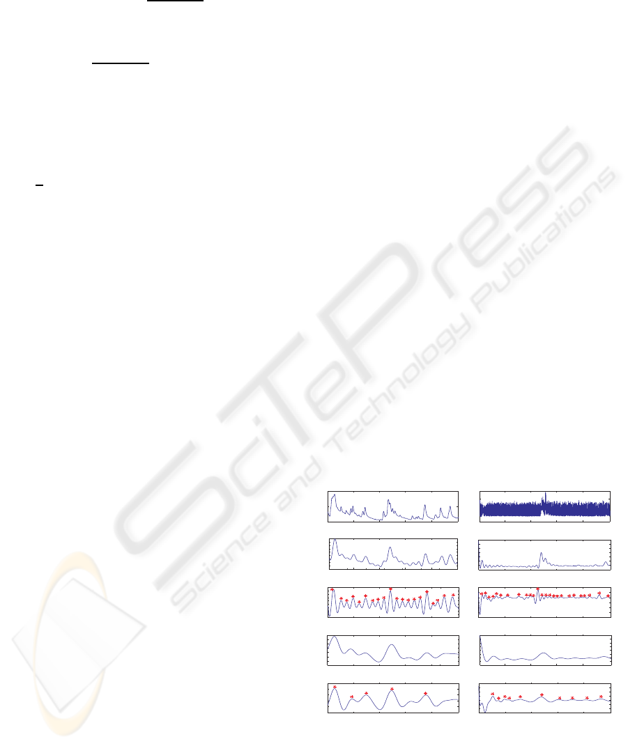
4.2.3 Skin Conductivity (SC)
The mean value, standard deviation, and mean of first
and second derivations are extracted as features from
the normalized SC signal and the low-passed SC sig-
nal using 0.2 Hz of cutoff frequency. To obtain a de-
trended SCR (skin conductance response) waveform
without DC-level components, we removed continu-
ous, piecewise linear trend in the two low-passed sig-
nals, i.e., very low-passed (VLP) with 0.08 Hz and
low-passed (LP) signal with 0.2 Hz of cutoff fre-
quency, respectively (see Fig. 6 (a)-(e)).
The baseline of the SC signal was calculated and
subtracted to consider only relative amplitudes. By
0
15
20
25
-2
-1
0
1
2
3
4
5
6
-3
-2
-1
0
1
2
3
4
-0.06
-0.04
-0.02
0
0.02
0.04
0.06
0.08
0.1
-2
-1
0
1
2
3
2
4
6
8
-0.5
0
0.5
1
1.5
2
2.5
3
-0.15
-0.1
-0.05
0
0.05
0.1
0.15
0.2
-1.5
-1
-0.5
0
0.5
1
-0.5
0
0.5
1
1.5
2
2.5
3
(a) SC_raw signal (f) EMG_raw signal
(b) SC_lowpassed, fc=0.2Hz (g) EMG_lowpassed, fc=0.3Hz
(c) SC_detrended, #occurrence (h) EMG_detrended, #occurrence
(d) SC_vlowpassed, fc=0.08Hz (i) EMG_vlowpassed, fc=0.08Hz
(e) SC_detrended, #occurrence (j) EMG_detrended, #occurrence
0
0
1000 2000 3000 4000 5000
0 1000 2000 3000 4000 5000
0 1000 2000 3000 4000 5000
0 1000 2000 3000 4000 5000
0 1000 2000 3000 4000 5000
0 1000 2000 3000 4000 5000
0 1000 2000 3000 4000 5000
0 1000 2000 3000 4000 5000
0 1000 2000 3000 4000 5000
1000 2000 3000 4000 5000
Figure 6: Analysis Examples of SC and EMG signals.
finding two consecutive zero-crossings and the maxi-
mum value between them, we calculated the number
of SCR occurrences within 100 seconds from each LP
and VLP signal, mean of the amplitudes of all occur-
BIOSIGNALS 2008 - International Conference on Bio-inspired Systems and Signal Processing
128

rences, and ratio of the SCR occurrences within the
low-passed signals (VLP/LP).
4.2.4 Electromyography (EMG)
For the EMG signal we calculated similar types of
features as in the case of the SC signal. From normal-
ized and low-passed signals, the mean value of entire
signal, the mean of first and second derivations, and
the standard deviation are extracted as features. The
occurrence number of myo-responsesand ratio of that
within VLP and LP signals are also added in feature
set by similar manner used for detecting the SCR oc-
currence but with 0.08 Hz (VLP) and 0.3 Hz (LP) of
cutoff frequency (see Fig. 6.(f)-(j)).
Finally we obtained a total of 110 features from
the 4-channel biosignals; 53 (ECG) + 37 (RSP) + 10
(SC) + 10 (EMG).
5 CLASSIFICATION RESULT
For classification we used the pseudoinverse linear
discriminant analysis (pLDA) (Ye and Li, 2005),
combined with the sequential backward selection
(SBS) (Kittler, 1986) to select significant feature sub-
set. The pLDA is a natural extension of classical
LDA by applying eigenvalue decomposition to the
scatter matrices, in order to deal with the sigular-
ity problem of LDA. Table 1 with confusion ma-
trix presents the correct classification ratio (C CR ) of
subject-dependent (Subject A, B, and C) and subject-
independent (All) classification where the features of
all the subjects are simply merged and normalized.
We used leave-one-out cross-validation where a sin-
gle observation taken from the entire samples is used
as the test data and the remaining observations are
used for training the classifier. This is repeated such
that each observation in the samples is used once as
the test data. In the Table, it turned out that the C CR
is depending on subject to subject. For example, best
accuracy was 91% from subject B and lowest was
81% from subject A. Not only the overall accuracy but
the C C R of the single emotions differs from subject
to subject. On the other side, it is very meaningfulthat
relatively robust recognition accuracy is achieved for
the classification between emotions that are recipro-
cal with each other regarding the diagonal quadrants
in the 2D emotion model, i.e., joy vs. sadness and
anger vs. pleasure. Moreover, the accuracy is much
better than that of arousal classification.
The C C R of subject-independent classification
was not comparable to that obtained for subject-
dependent classification. As shown in Figure 7, merg-
Table 1: Recognition results in rates (error 0.00 = C CR
100%) achieved by using pLDA with SBS and leave-one-
out cross validation.
# of samples: 120 for each subject and 360 for All.
Subject A (CC R % = 81%)
joy anger sadness pleasure total* error
joy 22 4 1 3 30 0.27
anger 3 26 1 0 30 0.13
sadness 1 2 23 4 30 0.23
pleasure 3 0 1 26 30 0.13
Subject B (CC R % = 91%)
joy anger sadness pleasure total* error
joy 27 3 0 0 30 0.10
anger 3 25 1 1 30 0.17
sadness 0 2 28 0 30 0.07
pleasure 0 1 0 29 30 0.03
Subject C (CC R % = 89%)
joy anger sadness pleasure total* error
joy 28 0 2 0 30 0.07
anger 0 30 0 0 30 0.00
sadness 0 0 24 6 30 0.20
pleasure 0 0 5 25 30 0.17
All: Subject-independent (C CR % = 65%)
joy anger sadness pleasure total* error
joy 62 9 8 11 90 0.31
anger 15 57 13 5 90 0.37
sadness 9 6 58 17 90 0.36
pleasure 8 5 21 56 90 0.38
*: Actual total # of samples
ing the features of all subjects does not refine the dis-
criminating information related to the emotions, but
rather leads to scattered class boundaries.
We also tried to differentiate the emotions based
on the two axes, arousal and valence, in the 2D emo-
tion model. The samples of four emotions are di-
vided into groups of negative valence (anger/sadness)
and positive valence (joy/pleasure) and into groups
of high arousal (joy/anger) and low arousal (sad-
ness/pleasure). By using the same methods, we then
performed two-class classification of the dividedsam-
ples for arousal and valence separately. Finally, it
turned out that emotion-relevant ANS specificity can
be observed more conspicuously in the arousal axis
regardless of subject-dependent or independent case.
Classification of arousal achievedan acceptable C CR
of 97-99% for the subject-dependent recognition and
89% for the subject-independent recognition, while
the results for valence were 88-94% and 77%, respec-
tively.
MULTI-CHANNEL BIOSIGNAL ANALYSIS FOR AUTOMATIC EMOTION RECOGNITION
129
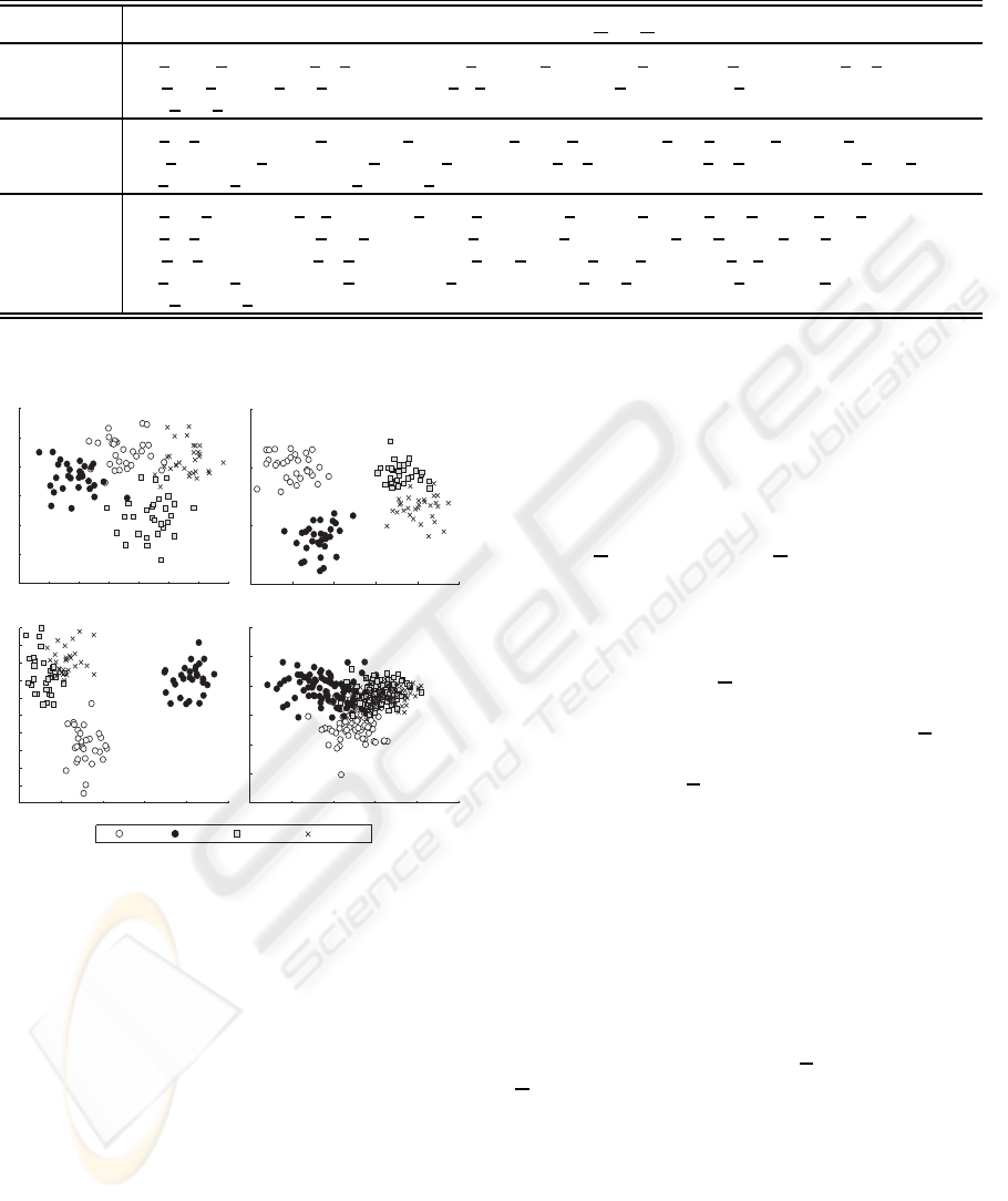
Table 2: Best emotion-relevant features extracted from four channel physiological signals. Arousal classes:
joy+anger/sadness+pleasure, Valence classes: joy+pleasure/anger+sadness, Four classes: joy/anger/sadness/pleasure.
Classes Best Emotion-relevant Features
(Ch value domain,
C
: ECG,
R
: RSP,
S
: SC,
M
: EMG)
Arousal C std(diff) HRVtime, C sd2 PoincareHRV, C powerLow HRVspec, R meanEnergy SubSpectra, R sd2 PoincareBRV
R mean MSE, S mean RawLowpassed, S std RawLowpassed, M #occurrenceRatio RawLowpassed
M mean RawNormed
Valence C sd2 PoincareHRV, C meanEnergy SubSpectra, C ratioLH HRVspec, C mean MSE, C mean(diff) MSE
R meanEnergy SubSpectra, R mean(diff) SubSpectra, R sd1 PoincareBRV, R sd2 PoincareBRV, R mean MSE
S mean(diff) RawNormed, M mean(diff) RawNormed
Four Emotions C mean HRVtime, C std HRVtime, C std(diff) HRVtime, C mean(diff) MSE, C mean MSE, C mean SSE
C sd2 PoincareHRV, C mean SubSpectra, R meanEnergy SubSpectra, R mean SSE, R mean BRVtime
R sd1 PoincareBRV, R sd2 PoincareBRV, R mean MSE, R power BRVspec, S std RawLowpassed
S mean(diff) RawNormed, S mean(diff(diff)) RawLowpassed, S mean RawNormed, S #occurrence RawLowpassed
M mean(diff) RawNormed
: overall selected features are printed in bold
2.4 2.6 2.8 3 3.2 3.4
x 10
-3
-6.5
-6.4
-6.3
-6.2
-6.1
-6
-5.9
-5.8
-5.7
-5.6
-5.5
x 10
-3
1.36 1.37 1.38 1.39 1.4 1.41 1.42 1.43
x 10
-3
0.0221
0.0222
0.0223
0.0224
0.0225
0.0226
0.0227
-20 -15 -10 -5 0 5
x 10
-6
5.5
5.55
5.6
5.65
x 10
-3
-5.6 -5.5 -5.4 -5.3 -5.2 -5.1
x 10
-4
-9.5
-9
-8.5
-8
-7.5
-7
-6.5
x 10
-4
joy
anger
sadness
pleasure
(a) (b)
(d)(c)
Figure 7: Comparison of feature distributions of subject-
dependent and subject-independent case. (a) Subject A, (b)
Subject B, (c) Subject C, (d) Subject-independent.
6 BEST EMOTION-RELEVANT
ANS FEATURES
In Table 2, the best emotion-relevant features, that
we determined by ranking the features selected for
all subjects (including Subject All) in each classi-
fication problem, are listed in detail by specifying
their values and domains. One interesting result is
that each classification problem respectively links to-
gether with certain feature domain. The features ob-
tained from time/frequency analysis of HRV time se-
ries are decisive for arousal and four emotions clas-
sification, while the features from MSE domain of
ECG signals are a predominant factor for correct va-
lence differentiation. Particularly, mutually sympa-
thizing correlate between HRV and BRV which is
firstly proposed in this paper has been clearly ob-
served in all the classification problems by the fea-
tures from their time/frequency analysis and Poincar´e
domain,
PoincareHRV and PoincareBRV. This re-
veals a manifest cross-correlation between respiration
and cardiac activity with respect to emotional state.
Furthermore, the correlation between heart rate and
respiration is obviously captured by the features from
HRV power spectrum (
HRVspec), the fast/long-term
HRV/BRV analysis using Poincar´e method, and the
multiscale variance analysis of HRV/BRV (
MSE),
and that the peaks of high frequency range in HR
subband spectrum (
SubSpectra)provide information
about how the sinoatrial node responds to vagal activ-
ity at certain respiration frequency.
In addtion, we analyzed the number of selected
features for the three classification problems, arousal,
valence, and four emotion states. For the arousal
classification, relatively few features are used but
achieved higher recognition accuracy compared to
the other class problems. After the ratio of num-
ber of selected features to the total feature number
of each channel, it was obvious that the SC and
EMG activities reflected in both
RawLowpassed and
RawNormed domains (see Table 2) are more signif-
icant for arousal classification than the other chan-
nels. This supports also the experimental elucidation
in previous works that the SCR is linearly correlated
with the intensity of arousal. On the other side, we
could observe a remarkable increase of number of the
ECG and RSP features for the case of valence classi-
fication.
BIOSIGNALS 2008 - International Conference on Bio-inspired Systems and Signal Processing
130

7 CONCLUSIONS
In this paper, we treated all essential stages of auto-
matic emotion recognition system using multichannel
physiological measures, from data collection up to
classification process, and analyzed the results from
each stage of the system. For four emotional states of
three subjects, we achieved average recognition accu-
racy of 91% which connotes more than a prima fa-
cie evidence that there exist some ANS differences
among emotions.
A wide range of physiological features from var-
ious analysis domains including time, frequency, en-
tropy, geometric analysis, subband spectra, multiscale
entropy, and HRV/BRV has been proposed to search
the best emotion-relevant features and to correlate
them with emotional states. The selected best fea-
tures are specified in detail and their effectiveness is
proven by classification results. We found that SC
and EMG are linearly correlated with arousal change
in emotional ANS activities, and that the features in
ECG and RSP are dominant for valence differentia-
tion. Particularly, the HRV/BRV analysis revealed the
cross-correlation between heart rate and respiration.
As we humans use several modalities jointly to in-
terpret emotional states since emotion affects almost
all modes, one most challenging issue in near future
work is to explore multimodal analysis for emotion
recognition. Toward the human-likeanalysis and finer
resolution of recognizable emotion classes, an essen-
tial step would be therefore to find innate priority
among the modalities to be preferred for each emo-
tional state. In this sense, physiological channel can
be considered as a “baseline channel” in designing
a multimodal fashion of emotion recognition system,
since it provides several advantages over other exter-
nal channels and acceptable recognition accuracy, as
we presented in this work.
ACKNOWLEDGEMENTS
This research was partially supportedby the European
Commission (HUMAINE NoE: FP6 IST-507422).
REFERENCES
Costa, M., Goldberger, A. L., and Peng, C.-K. (2005). Mul-
tiscale entropy analysis of biological signals. Phys.
Rev., E 71(021906).
Cowie, R., Douglas-Cowie, E., Tsapatsoulis, N., Votsis,
G., Kollias, S., Fellenz, W., and Taylor, J. G. (2001).
Emotion recognition in human-computer interaction.
IEEE Signal Processing Mag., 18:32–80.
Gross, J. J. and Levenson, R. W. (1995). Emotion elicitation
using films. Cognition and Emotion, 9:87–108.
Healey, J. and Picard, R. W. (1998). Digital processing of
affective signals. In Proc. IEEE Int. Conf. Acoust.,
Speech, and Signal Proc., pages 3749–3752, Seattle,
WA.
Kamen, P. W., Krum, H., and Tonkin, A. M. (1996).
Poincare plot of heart rate variability allows quantita-
tive display of parasympathetic nervous activity. Clin.
Sci., 91:201–208.
Kim, K. H., Bang, S. W., and Kim, S. R. (2004). Emo-
tion recognition system using short-term monitoring
of physiological signals. Medical & Biological Engi-
neering & Computing, 42:419–427.
Kittler, J. (1986). Feature Selection and Extraction, pages
59–83. Academic Press, Inc.
LeDoux, J. E. (1992). The Amygdala: Neurobiological As-
pects of Emotion, Memory, and Mental Dysfunction,
pages 339–351. New York: Wiley-Liss.
Malliani, A. (1999). The pattern of sympathovagal balance
explored in the frequency domain. News Physiol. Sci.,
14:111–117.
Nasoz, F., Alvarez, K., Lisetti, C., and Finkelstein, N.
(2003). Emotion recognition from physiological sig-
nals for presence technologies. International Journal
of Cognition, Technology, and Work - Special Issue on
Presence, 6(1).
Pan, J. and Tompkins, W. (1985). A real-time qrs detection
algorithm. IEEE Trans. Biomed. Eng., 32(3):230–323.
Picard, R., Vyzas, E., and Healy, J. (2001). Toward machine
emotional intelligence: Analysis of affective physio-
logical state. IEEE Trans. Pattern Anal. and Machine
Intell., 23(10):1175–1191.
Richmann, J. and Moorman, J. (2000). Physiological time
series analysis using approximate entropy and sam-
ple entropy. Am. J. Physiol. Heart Circ. Physiol. 278,
H2039.
Ye, J. and Li, Q. (2005). A two-stage linear discriminant
analysis via qr-decomposition. pami, 27(6).
MULTI-CHANNEL BIOSIGNAL ANALYSIS FOR AUTOMATIC EMOTION RECOGNITION
131
