
ENHANCED ANALYSIS OF UTERINE ACTIVTY USING SURFACE
ELECTROMYOGRAPHY
A. Herzog, L. Reicke, M. Kr¨oger
Institute of Dynamics and Vibration Research, Leibniz University Hannover, Germany
C. Sohn, H. Maul
Obstetrics and Gynecology, UniversityHospital Heidelberg, Germany
Keywords:
Uterine, electromyography, pulse detection, stochastic analysis, Karhunen-Lo`eve, principal component.
Abstract:
This contribution presents a new approach for the enhanced analysis of uterine surface electromyography
(EMG). First, a pulse detection separates the pulses, which contain the essential information about the uterine
contractibility, from the flat line sections during relaxation. The functionality of this semi-automatic algorithm
is controlled by two comprehensible parameters. Subsequently, the mean frequency, which serves as a crite-
rion for imminent delivery, is evaluated from the extracted pulses. Although the pulse detection reduces the
deviation of the mean frequency significantly, the results are still sensitive to parameter variations in the pulse
detection. A stochastic analysis based on the Karhunen-Lo`eve transform (KLT) derives generalised patterns,
the eigenforms, from the pulse ensemble. The mean frequency of the first eigenform is less sensitive to pa-
rameter variations. Additionally, the correlation between the eigenforms of the left and right surface electrode
can serve as a criterion for the measurement’s quality.
1 INTRODUCTION
Even in modern obstetrics, the point of delivery can-
not be precisely predicted. Although the majority
of pregnancies passes without any complications, the
significance of an enhanced analysis of uterine activ-
ity arises from the diagnosis of preterm labor as well
as the treatment of delayed delivery.
The uterine muscle (myometrium), which has
maintained a quiescent state during the majority of
pregnancy, is prepared for labor by local contractions.
These contractions, called training labors, improve
the synchronisation between the single muscle cells
in order to obtain a defined contraction sequence dur-
ing delivery. Therefore, the identification of imminent
labor requires an elaborate analysis and interpretation
of this preparatory phase.
Several methods for the evaluation of uterine con-
tractibility are commonly used: TOCO, IUPC and
EMG. Uterine contractions cause variations in the
abdomen’s contour, which can be detected by pres-
sure sensors. Due to the indirect measurement, this
so-called external tocodynamometry (TOCO) is not
sensitive and reliable enough. A more reliable ap-
proach consists of measuring the uterine’s internal
pressure (intrauterine pressure catheter, IUPC). The
surface electromyography (EMG) combines the non-
invasiveness property of TOCO with a sensitivity sim-
ilar to that of the IUPC (Maul et al., 2004). The
muscular activity is accompanied by variations of the
electric potential at the neuromuscular junction be-
tween nerve and muscle cells. This potential can
be picked up directly by needle electrodes and range
from −70mV (relaxation) up to +30mV during con-
traction. In case of surface electrodes, the voltage has
to be transmitted via the tissue to the skin, yielding to
lower peak values as well as deformations in the time
history of the voltage signal. For the measurement
of the uterine contractions two surface electrodes are
used. They are located on the right and left side of the
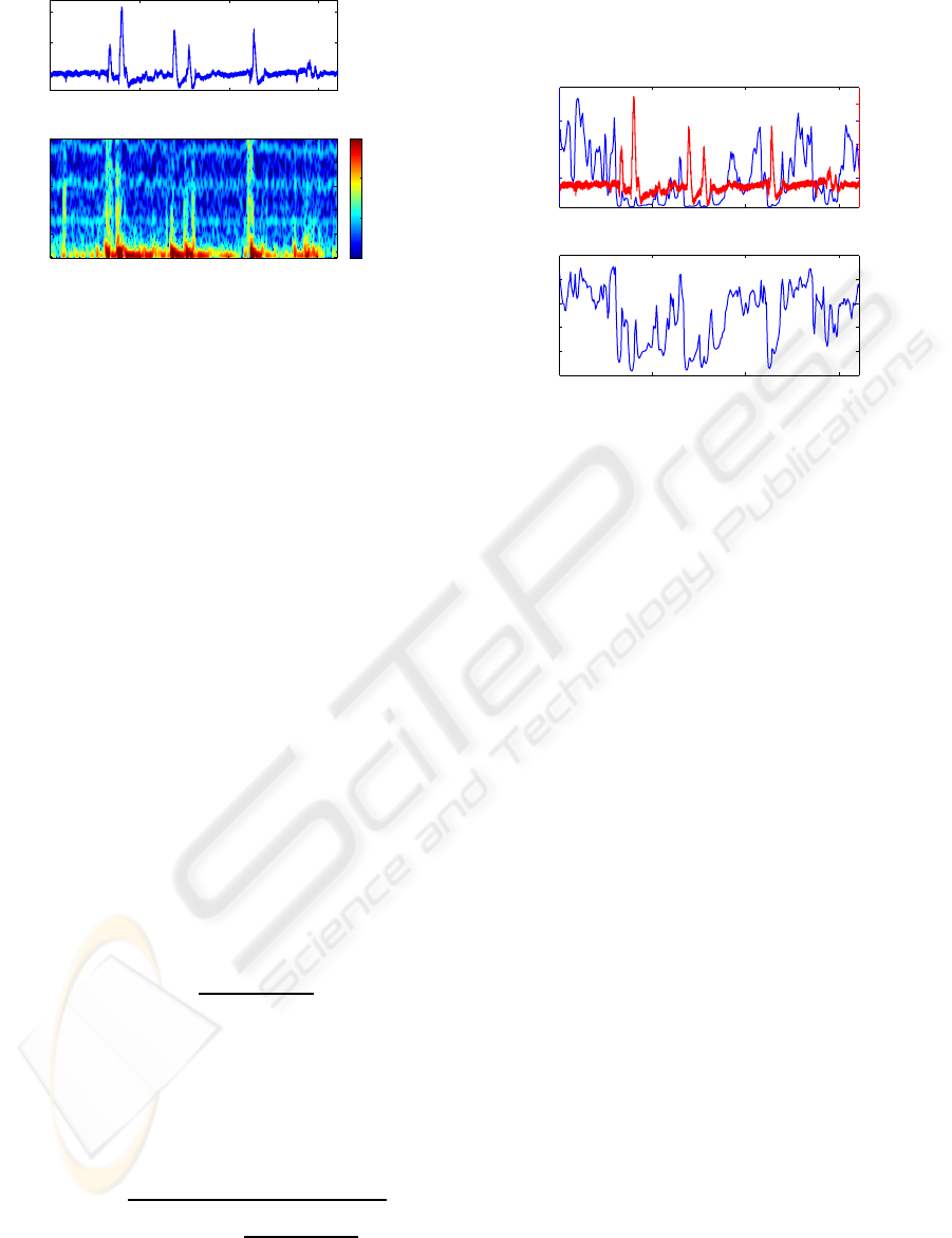
abdomen. The time-history of a single electromyo-
gram (EMG)-signal is displayed in Figure 1 above.
The pulses, which belong to uterine contractions, are
separated by flat line sections. Up to now, the fre-
quency characteristics have been derived from large
sections of its time history by means of the Fourier
transform. Based on the assumption that ongoing syn-
chronisation leads to an increase of the pulse’s attack
377
Herzog A., Reicke L., Kröger M., Sohn C. and Maul H. (2008).
ENHANCED ANALYSIS OF UTERINE ACTIVTY USING SURFACE ELECTROMYOGRAPHY.
In Proceedings of the First International Conference on Bio-inspired Systems and Signal Processing, pages 377-384
DOI: 10.5220/0001062903770384
Copyright
c
SciTePress
0 100 200 300
0
2
4
level [mV]
time [s]
frequency [Hz]
log10 [1mV]
0 100 200 300
0
1
2
3
4
5
−3
−2
−1
0
Figure 1: Surface Electromyogram: Time history (above)
and its short-time Fourier transform (below).
and decay slope, the mean frequencyof the calculated
spectrum serves as a criterion to judge imminent de-
livery.
But a detailed analysis in the time-frequency do-
main reveals a strongly varying frequency content.
This analysis is done by a discrete short-time Fourier
transform (STFT) based on a Hann-Window 5s long.
An additional zero-padding and a logarithmic scal-
ing of the resulting amplitude-coefficients unveils all
the significant details. An introduction into the time-
frequencytransforms can be foundin (Mertins, 1999),
practical aspects are discussed e.g. in (Reicke et al.,
2006).
The logarithmic representation of the STFT co-
efficients in Figure 1 does not only show the broad
frequency content of the pulses, it even unveils the
heart beat of the foetus at 1.6Hz as well as its harmon-
ics. Due to the fact that the pulses rather than the flat
line sections contain the information about the uterine
contractibility, the authors suggest an enhanced anal-
ysis which is restricted to the EMG-pulses. This new
approach is supported by Figure 2. The diagram on
the top shows the instantaneous mean frequency
f
m
(t) =
∞
Z
0
f ·
|X
STFT
( f,t)|
2
||X
STFT
(t)||
2
df (1)
derived from the amplitude coefficients X
STFT
( f,t) of
the STFT. The norm ||X
STFT
(t)|| denotes the instanta-
neous energy
R
|X
STFT
( f,t)
2
|df of the STFT. The red
line represents the level of the original EMG-signal.
The lower diagram shows the evolution of the mean
frequency’s standard deviation
σ
f
(t) =
v
u
u
t
∞
Z
0
( f − f
m
)
2
·
|X
STFT
( f,t)|
2
||X
STFT
(t)||
2
df (2)
over time. It underlines that a reliable estimation of
the mean frequency is restricted to the pulses. Only
in these time intervals, the standard deviation is less
than 3Hz.
0 100 200 300
0
10
20
30
mean freq. [Hz]
0 100 200 300
0
2
4
level [mV]
0 100 200 300
0
5
10
15
20
time [s]
std. dev. [Hz]
Figure 2: Instantaneous mean frequency (above) and its
standard deviation (below) of the signal shown in Fig. 1.
As only the pulses contain the relevant informa-
tion, it is convenient to analyse the pulses without
the intervals of relaxation. This contribution presents
a semi-automatic pulse detection, which extracts the
pulses out of the measured EMG-signal. The expres-
sion semi-automatic underlines that the operation is
controlled by the physician, whereas the algorithm
undertakes the time-consuming and exhausting work
of scanning through the signal searching for pulses.
Additionally, the use of surface electrodes causes de-
formations of the pulse shape. Therefore, the pulses
are processed by a stochastic method based on the
Karhunen-Lo`eve transform to evaluate a generalised
pattern.
2 PULSE DETECTION
2.1 Conditioning
The surface-EMG signals are distorted by noise and
a low frequency drift. A low-pass filter, which rejects
frequencies higher than 7.5Hz, is applied to attenu-
ate the noise. The low frequency drift is reduced by a
high-pass filter with a cut-off frequency of 0.1Hz and
a transition band of 0.2Hz. Both are implemented as
finite impulse response (FIR) filters based on a Kaiser
window design (Oppenheim and Schafer, 1999). An
additional noise-reduction is achieved by the pulse
detection: the flat line intervals, which are charac-
terised by a low signal-to-noise ratio, are excluded
from the further analysis.
BIOSIGNALS 2008 - International Conference on Bio-inspired Systems and Signal Processing
378
2.2 Pulse Detection
The pulse detection extracts those parts of the sig-
nal which contain the relevant information about the
uterine contractibility. The localisation of the pulses
is done regarding the magnitude of the signal. First,
the global maximum and the mean value of the sig-
nal’s magnitude as an approximation of the noise level
are determined. All local peaks in the range between
these two values can be considered as potential pulse
centres. But only pulses whose peak values largely
exceed the noise limit offer a sufficient signal-to-noise
ratio. Therefore, the first parameter of the pulse detec-
tion, the level value, is introduced. This value deter-
mines the percentage of the range between noise level
and global maximum which is added to the noise level
in order to define the lower level limit. If the level
value is chosen equal to zero, the lower level limit is
identical to the noise level. Hence, any peak value
higher than the noise level is considered as a pulse
centre. In case of a level value equal to ”1”, the lower
level limit reaches the global maximum and any peak
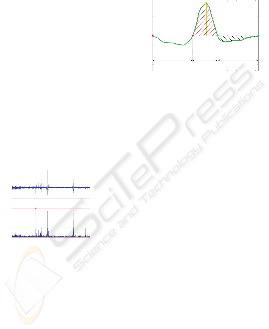
except for the global maximum will be rejected. Fig-
ure 3 shows a particular lower level limit which cor-
responds to a level value of 0.3.
0
2
4
-2
6
6
4
2
0
0
0
1000
1000
2000
2000
3000
3000
time[s]
level[mV]
level[mV]
global
maximum
noiselevel
lowerlevel
limit
Figure 3: EMG-signal (above) and its magnitude with
global maximum, noise level and a particular level value.
After the localisation of the pulse centres in the
signal, the initial and end point of each pulse are de-
termined. The pulse detection is based on the assump-
tion that a pulse begins and ends at roots. Therefore,
any low frequent drift has to be removed (cp. 2.1)
before the execution of the pulse detection algorithm.
Starting with the pulse centre, the adjoining roots tem-
porary describe the initial and end points. In the fol-
lowing, this part of the pulse between these two roots
is called the inner pulse. If these points were finally
considered as the pulse’s initial and end points, ad-
jacent over- and undershoots, which might belong to
the pulse and therefore contain valuable information,
would not be extracted. Hence, the surroundings of
the inner pulse have to be taken into consideration.
0
1
-1
3190
3195
3200
time[s]
level[mV]
inner
pulse
undershoot
undershoot
Figure 4: Evaluation of inner and outer area.
Figure 4 displays a pulse with a preceding and
subsequent undershoot. To determine whether these
undershoots are part of the pulse, the roots before and
after the temporary initial and end points are consid-
ered. For example, the temporary end point and the
root located on its right enclose the subsequent under-
shoot. Now, the area of the undershoot is calculated
and related to the area of the inner pulse. In Figure 4,
the area of the undershoot (”outer area”) and the in-
ner pulse (”inner area”) are hatched in black and red,
respectively. If the ratio of the outer and inner area
exceeds a given value, the corresponding undershoot
belongs to the pulse. If the right undershoot in Figure
4 fulfils this area criterion, the inner pulse is expanded
by the right undershoot and the temporary end point
is shifted by one root to the right.
This given value is called the area value and can
be chosen anywhere between ”0”, which connects any
adjacent undershoot to the inner pulse, and ”1”. In
case of an area value equal to ”1”, only undershoots
exhibiting an area greater than the inner area are at-
tached to the pulse. The same procedure is done with
the undershoot on the left. This algorithm goes on
in both directions until the area of the current over-
or undershoot is less than that of the original inner
pulse. In this case, the temporary root becomes the
final root, which borders the pulse to one side. As
soon as the left and right final roots are determined,
the pulse can be extracted from the signal. The de-
tection of the next pulses follows the same algorithm.
In order to avoid overlapping of closely neighbouring
pulses, the extracted pulse data are replaced by zeros.
The level value influences the quantity of detected
pulses. The lower the level value, the more peaks
of the signal are regarded as pulse centres. The area
value controls the lengths of the pulses. The greater
the area value, the less over- and undershoots belong
to the inner pulse and therefore the less pulses are
ENHANCED ANALYSIS OF UTERINE ACTIVTY USING SURFACE ELECTROMYOGRAPHY
379
lengthened beyond their inner pulse. However, the
area value has an influence on the quantity of the
pulses, too. If the area value is very low, the pulses
extracted from the signal are so long that less pulses
can be detected in the remaining signal parts.
2.3 Characteristic Values
The pulse detection scans through the signal and cuts
out single time histories belonging to those pulses
whose shapes match the pattern specified by the level
and area value. The extracted pulses are described
in the time domain by their peak values and lengths.
Additionally, each pulse is analysed in the frequency
domain by the discrete Fourier transform (DFT). Con-
trary to the short-time Fourier transform X
STFT
( f,t)
of the entire signal, the spectrum X
pulse
( f) of an indi-
vidual pulse is not time-dependent. Hence, each pulse
is characterised by two values in the frequency do-
main, the mean frequency f
m
and the variance σ
2
f
.
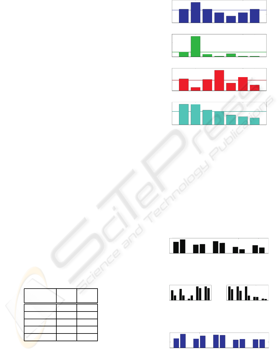
Based on a measured EMG-signal, Figure 5 shows
the characteristic values of those pulses that fulfill a
level value equal to ”0.3”, i.e. 30 % of the global max-
imum, and an area value of ”0.4”. In the diagrams, the
horizontal line denotes the arithmetic mean. The third
diagram exhibits a strong variation in the pulse length.
Particularly, the 2nd and 4th pulse length strongly
deviate from the mean of ≈ 650samples. The 2nd
pulse’s mean frequency f
m
largely exceeds the mean
of ≈ 0.16Hz. The reason may be the short duration
of ≈ 200Samples, which also increases the variance
σ
2
f
.
In order to demonstrate the influence of the two
parameters level value and area value on the num-
ber, length and mean frequencyof the pulses extracted
from the EMG-signal, the results of five different
pairs, shown in Table 1, are compared in Figures 6,
7 and 8.
Table 1: Pairs of parameters used for pulse detection.
parameter level area
settings value value
E1 0.05 0.1
E2 0.1 0.1
E3 0.1 0.3
E4 0.3 0.4
E5 0.3 0.7
For each pair, denoted with E1 up to E5, the left
and right bars represent the left and right channel of
the electromyogram, respectively. With increasing
level value, the number of pulses decreases because
pulses with lower peak values are now rejected. A
comparison between pair E2 and E3 as well as E4
0.2
0.1
0
0.04
0.02
0
1000
500
0
3
2
1
0
variance
[Hz]
2
length
[samples]
meanfrequency
[Hz]
peakvalues
[Hz]
1
2 3
4
5
6
7
1
2 3
4
5
6
7
1
2 3
4
5
6
7
1
2 3
4
5
6
7
pulses
Figure 5: Characteristic values of a pulse ensemble cut out
from a measured EMG-signal.
and E5 unveils the influence of the area value on the
length and numberof pulses. An increasing area value
leads to a shorter maximum pulse length. On the
other hand, a higher level value increases the mini-
mum pulse length because the pulses with low peak
values, which are obviously shorter, are not consid-
ered anymore. As it is mentioned in 2.2, a more re-
strictive area value can resolve and separate closely
neighbouring pulses into two individual pulse shapes.
20
10
0
E1
E2
E3 E4 E5
number
ofpulses
Figure 6: Influence of parameters in Table 1 on number of
pulses extracted.
200
100
0
length
[samples]
E1
E1
E2
E2
E3
E3
E4
E4
E5
E5
5000
0
Figure 7: Influence of parameters in Table 1 on minimum
and maximum pulse length.
0.2
0.1
0
E1
E2
E3
E4 E5
frequency
[Hz]
Figure 8: Influence of parameters in Table 1 on mean fre-
quency.
The variation of the pulse length takes effect on
the mean frequency, which is shown in Figure 8. It
BIOSIGNALS 2008 - International Conference on Bio-inspired Systems and Signal Processing
380
reveals a strong sensitivity of the mean frequency to
the given level and area values. This insufficient un-
certainty motivated the authors to improve the anal-
ysis by a stochastic signal processing, which is de-
scribed in the next section. Additionally, a criterion is
required to give reliable information about the qual-
ity of the signal. A straightforward approach is the
consideration of the signal-to-noise ratio, but this will
not take into account any correlation between the two
channels .
3 STOCHASTIC ANALYSIS
3.1 Karhunen-Lo
`
eve Transform
The electric potential, which occurs at a neuromuscu-
lar junction, is transmitted via a quite complex elec-
tric network to the two electrodes at the abdomen’s
surface. This leads to an amplitude attenuation of
≈ −20dB and deformations in the pulse shape. In ad-
dition, the location of the contraction is randomly dis-
tributed over the entire uterine muscle, which implies
a random distortion of the EMG-signal with regard to
the peak value and pulse shape.
Due to the fact that the measuring time of about
30min is very short compared to the ongoing preg-
nancy, a stationary stochastic process is assumed. The
individual pulse shapes extracted by the pulse detec-
tion are considered as the realisations of this stochas-
tic process. The new approach uses the Karhunen-
Lo`eve transform (KLT), also referred to as Principal
Component Analysis (PCA), to determine a charac-
teristic pulse shape out of the pulse ensemble.
The Karhunen-Lo`eve transform is a signal-
depending decomposition based on the covariance
matrix
R
˜x˜x
= E
˜x ˜x
T
, (3)
in which E{ } denotes the statistic expectation and ˜x
the stochastic process. The decomposition requires
the eigenvectors u of the eigenvalue problem
R
˜x˜x
u = λ u. (4)
The eigenvectors u can be regarded as the characteris-
tic shapes of the stochastic process. The eigenvalue λ
represents the degree of similarity between the corre-
sponding eigenvector and the individual pulses. In the
following, the product of eigenvector and eigenvalue
is denoted as eigenform. The more similar the individ-
ual pulses of the ensemble are to each other, the more
dominant becomes the first eigenform. If the ensem-
ble consists of identical pulse shapes, the first eigen-
value will contain the whole variance of the stochastic
process, while all other eigenvalues are equal to 0. A
brief introduction into the Karhunen-Lo`eve transform
is given in (Mertins, 1999), a detailed description can
be found in (Jolliffe, 2002).
0
2
4
6
8
10
12
2
4
6
2
1
0
-1
-2
-3
time [s]
pulses
level[mV]
Figure 9: Ensemble of centred pulses.
For the stochastic analysis, a preprocessing of the
pulses is necessary. The calculation of the covariance
matrix requires an identical length of all the pulse
shapes. Therefore, the pulses are centered with re-
gard to their centres of area, followed by padding ze-
ros on both sides to obtain an identical pulse length.
The result of this preprocessing is shown in Figure 9,
in which the longest pulse, the blue one, specifies the
dimension of the covariance matrix. The other pulse
shapes are shifted in such a way that all area centres
coincide.
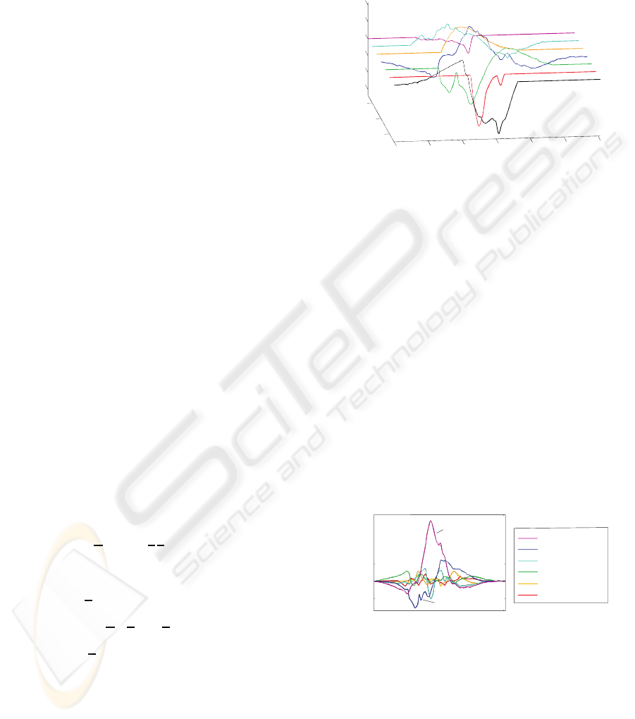
The result of the KLT of Figure 9 is displayed
in Figure 10: The first and second eigenforms (EF)
are dominant and contain ≈ 90% of the process’ vari-
ance. This can be seen from the time history on the
left side as well as the loadings on the right. In this
context, the loading denotes the normalised variance
of the stochastic process.
1.EF:67,13%
2.EF:22,51%
3.EF:4,66%
4.EF:2,67%
5.EF:1,81%
6.EF:0,82%
1,5
1
0,5
0
-0,5
level[mV]
2 4
6
8 10 12
time[s]
1.EF
2.EF
Figure 10: KLT: Eigenforms (left) and loadings (right).
Instead of deriving the mean frequency directly
from the pulse ensemble (cp. subsection 2.3), the
DFT of the first eigenform yields to a mean frequency
which is less sensitive to parameter variations. On
top of Figure 11, the global mean frequency, which
is evaluated as the arithmetic mean of the individual
eigenforms’ mean frequencies, is displayed accord-
ing to the parameter settings shown in Table 1. While
ENHANCED ANALYSIS OF UTERINE ACTIVTY USING SURFACE ELECTROMYOGRAPHY
381
the global mean frequency is susceptible to parameter
variations, the mean frequency derived from the first
eigenform seems to be less sensitive. Here, research
is in progress to confirm this observation.
0
0
0.1
0.1
0.2
0.2
E1
E1
E2
E2
E3
E3
E4
E4
E5
E5
frequency
[Hz]
frequency
[Hz]
Figure 11: KLT: global mean frequency (above) and mean
frequency of the first eigenform (below) for different pa-
rameter settings.
The Karhunen-Lo`eve transform does not only ex-
tract a characteristic pulse pattern, the first eigenform,
out of the pulse ensemble. It can also provide a reli-
able criterion of the electromyogram’s reliability. If
the first eigenvalue is dominant, the pattern of the first
eigenform is similar to the shapes of the majority of
pulses in the ensemble, while the other eigenforms
represent the deformations in the pulse shapes.
3.2 Correlation Analysis
So far, the two channels of the electromyogram have
been analysed separately. In case of a dominant
eigenvalue (see subsection 3.1), the corresponding
eigenform characterises the pulse pattern of the in-
dividual channel’s pulse ensemble very well. There-
fore, the correlation between the left and right EMG-
channel can be evaluated by regarding their first
eigenforms.
Even in case of identical pulse shapes, a time shift
between the left and right eigenform can occur. This
may be caused by different transmission delays from
the neuromuscular junction to the surface electrodes
in combination with the centring of the pulses before
the KLT is performed.
In order to evaluate the similarities between the
left and right eigenform u
ℓ
(t) and u
r
(t) the cross-
correlation function (CCF)
R
u
ℓ
u
r
(τ) =
∞
Z
−∞
u
ℓ
(t) · u
r
(t + τ) dt (5)
is used. If the two eigenforms are of identical shape
but shifted to each other, u
r
(t) = u
ℓ
(t − ∆t), the CCF
resembles an autocorrelation function (ACF) whose
maximum value is shifted along the time axis. Due
to the fact that an ACF is symmetric to its origin τ =
0, the CCF of two identical but shifted eigenforms is
symmetric with regard to the time shift ∆t:
R
u
ℓ
u
r
(∆t − τ) = R
u
ℓ
u
r
(∆t + τ). (6)
Because the eigenvector’s orientation is not specified
by Equation 4, the left and right eigenforms can dif-
fer in their signs. Therefore, maximum correlation in
the CCF appears at its global maximum or minimum.
First of all, the time shift of the CCF is determined by
its global extremum. Subsequently the CCF is divided
into a symmetric
R
symm
(τ) =
R
u
ℓ
u
r
(∆t + τ) + R
u
ℓ
u
r
(∆t − τ)
2
(7)
and antimetric
R
anti
(τ) =
R
u
ℓ
u
r
(∆t + τ) − R
u
ℓ
u
r
(∆t − τ)
2
(8)
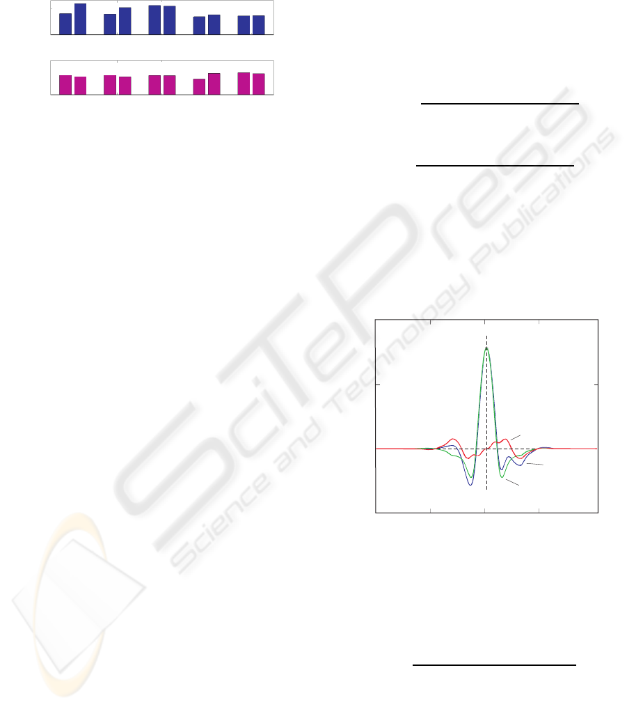
component. This decomposition is displayed in Fig-
ure 12. The extremum is located at ≈ 2000samples,
at which a vertical symmetry axis (dashed line) is
drawn. According to Equations 7 and 8 the cross-
correlation function (blue line) is decomposed into its
symmetric (green line) and antimetric (red line) com-
ponents.
0,02
0,01
0
-0,01
0
1000 2000
3000
CCF[Hz]
2
samples
CCF
antimetric
symmetric
Figure 12: Decomposition of the CCF (blue) at its ex-
tremum into a symmetric (green) and antimetric (red) com-
ponent.
Based on this decomposition a symmetry value
C
symm
= 1−
∞
R
−∞
R
u
ℓ
u
r
(τ) − R
symm
(τ)
2
dτ
∞
R
−∞
R
2
u
ℓ
u
r
(τ) dτ
(9)
can be specified as the square deviation of the CCF
from its symmetric component. In case of full axis
symmetry, the symmetric value in Equation 9 reaches
”1” or 100%. The cross-correlation function of the
left and right eigenforms for the parameter settings
BIOSIGNALS 2008 - International Conference on Bio-inspired Systems and Signal Processing
382
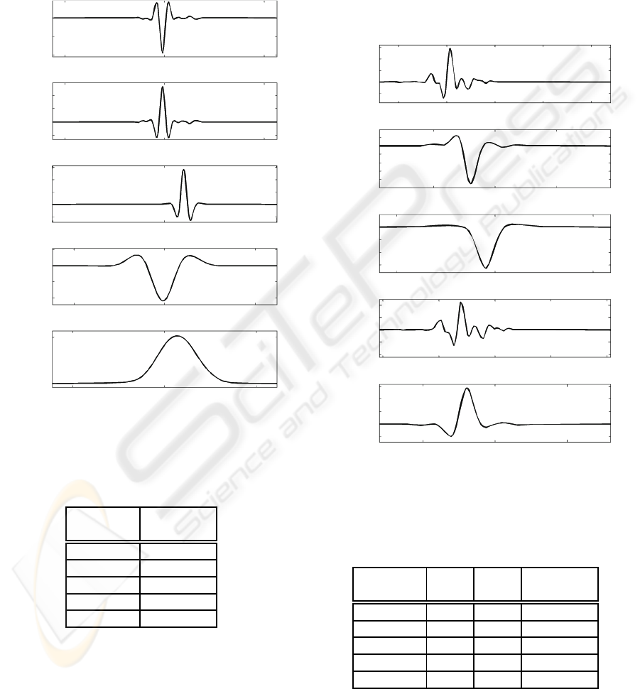
in Table 1 are displayed in Figure 13. The CCF’s
oscillations are caused by the under- and overshoots
of the EMG-pulses. With an increasing area value,
these parts diminish in the pulse shapes and eigen-
forms. The CCFs are dominated by their symmetric
components, which is also confirmed in Table 2 by
symmetry values close to 100%.
-50 0
50
-50 0
50
-50 0
50
0-10
10
0-5
5
lags[s]
0
-0.01
-0.02
CCF
E1
0.02
0
CCF
E2
0.02
0
CCF
E3
0
-0.2
CCF
E4
0.4
0.2
0
CCF
E5
Figure 13: Cross-correlation functions for the parameter
settings of Table 1.
Table 2: Symmetry values for parameter settings in Table 1.
parameter symmetry
settings value in %
E1 99.79
E2 99.74
E3 99.43
E4 99.97
E5 99.96
Figure 14 displays the eigenform’s cross-
correlation functions of another EMG-signal. The
eigenforms are based on a pulse detection whose
parameters are shown in Table 3. Due to a poorer
signal-to-noise ratio, the minimum level value is set
to 0.2. Only CCF
E8
, the CCF for the third parameter
set (level value of 0.2, area value equal to 0.7) seems
quite symmetric. This assumption is confirmed by a
symmetry value C
symm
= 0.9975 in Table 3.
This means that the eigenforms of the second
EMG-signal are more sensitive to variations of the
pulse detection’s parameters. This may be caused by
an incorrect application of the surface sensors, which
induces additional noise and deformations. There-
fore, the combination of the eigenforms’ loadings and
the symmetry value indicates the quality of the mea-
surement.
0
-40 40
0
-10
10
0
-10
10
0
-40
40
0
-10 10
lags[s]
0.02
0
CCF
E6
0
-0.4
-0.8
CCF
E7
0
-0.1
CCF
E8
0.4
0
-0.4
CCF
E9
0.1
0
CCF
E10
Figure 14: Cross-correlation function of another EMG-
signal with parameter settings of Table 3.
Table 3: Symmetry values of the second EMG-signal.
parameter level area symmetry
settings value value value in %
E6 0.2 0.1 86.29
E7 0.2 0.4 97.16
E8 0.2 0.7 99.75
E9 0.3 0.1 77.23
E10 0.3 0.4 96.19
ENHANCED ANALYSIS OF UTERINE ACTIVTY USING SURFACE ELECTROMYOGRAPHY
383

4 CONCLUSIONS
The existing methods for the analysis of EMG-signals
are not precise enough for a reliable prediction of
the point of delivery. The new approach presented
in this contribution is based on the distinction be-
tween pulses (muscular contraction) and flat line sec-
tions during relaxation. A time-frequncy analysis re-
veals that only the pulses contain relevant information
whereas the flat line sections can be neglected. For
this reason, a semi-automatic pulse detection is de-
veloped. The physician controls the functionality of
the pulse detection by adapting two comprehensible
parameters, while the time-consuming work of pulse
extraction is done automatically. The first parame-
ter, the level value, influences the number of extracted
pulses, whereas the second parameter, the area value,
determines the length of the pulses. Therefore, the
physician integrates his current observations as well
as his medical experiences into the pulse detection.
The use of surface electrodes leads to deforma-
tions in the individual pulse shapes. In this ap-
proach, the pulses extracted by the pulse detection
are treated as realisations of a stationary stochastic
process. In order to derive a generalized pattern, a
stochastic analysis, the Karhunen-Lo`eve-Transform
(KLT), is carried out. The KLT is based on the eigen-
value/eigenvector problem of the covariance matrix.
While an eigenvector represents a generalised pattern,
the corresponding eigenvalue specifies the degree of
similarity with regard to the pulse ensemble. Eigen-
value and eigenvector yield to the eigenform. The
more dominant the first eigenform is, the better it rep-
resents the pulses of the ensemble.
Until now, the mean frequency has been used for
the prediction of the point of delivery. Although the
pulse detection reduces the frequency deviation sig-
nificantly, the mean frequency remains sensitive to
variations of the pulse detection’s parameters because
the individual pulses are randomly distorted by con-
ductivity effects. The first eigenform of the KLT is
less susceptible to parameter variations. Particular
in case of a dominant first eigenform, the mean fre-
quency becomes a reliable criterion.
Furthermore, a new characteristic value is devel-
oped: the symmetry value. It is derived from the
cross-correlation function of the first eigenforms of
the left and right EMG-channel. If the quality of
the electromyogram is high, the pulse ensembles of
the left and right channel will yield to quite identical
eigenforms and a symmetry value close to 100%. To-
gether with the eigenvalues of the KLT, the symmetry
value serves as a criterion for the measurement’s reli-
ability.
In the future, the pulse detection combined with
the stochastic analysis will be applied on a sufficiently
large amount of electromyograms taken from various
women during the last period of pregnancy. With
these results, the reliability of this new approach as
well as the improvement with regards to the present
methods will be be quantified.
REFERENCES
Jolliffe, I. T. (2002). Principal Component Analysis.
Springer, New York, 2nd edition.
Maul, H., Maner, W. L., Olson, G., Saade, G. R., and
Garfield, R. E. (2004). Non-invasive transabdominal
uterine electromyography correlates with the strength
of intrauterine pressure and is predictive of labor
and delivery. In The Journal of Maternal-Fetal and
Neonatal Medicine. Parthenon Publishing.
Mertins, A. (1999). Signal analysis: wavelets, filter banks,
time-frequency transforms and applications. Wiley,
Chichester, 2nd edition.
Oppenheim, A. and Schafer, R. W. (1999). Discrete-time
signal processing. Prentice Hall, Upper Saddle River,
NJ, 2nd edition.
Reicke, L., Kaiser, I., and Kroeger, M. (2006). Identifi-
cation of the running-state of railway wheelsets. In
ISMA2006, International Conference on Noise & Vi-
bration Engineering. Katholieke Universiteit Leuven,
Department of Mechanical Engineering.
BIOSIGNALS 2008 - International Conference on Bio-inspired Systems and Signal Processing
384
