
Texture Learning by Fractal Compression
Benoît Dolez
1,2
and Nicole Vincent
1
1
CRIP5-SIP, René Descartes University, 45 rue des Saints Pères
75006 Paris, France
2
SAGEM DS, 178 rue de Paris, 91344 Massy, France
Abstract. This paper proposes a texture learning method based on fractal com-
pression. This type of compression is efficient for extracting self-similarities in
an image. Square blocks are studied and similarities between them highlighted.
This allows establishing a score and thus a rating of the blocks. Selecting the
blocks that best encode the biggest part of the image or a texture leads to a da-
tabase of the most representative ones. The recognition step consists in labeling
blocks and pixels of a new image. The blocks of the new image are matched
with the ones of the different texture databases. As an application, we used our
method to recognize vegetation and buildings on aerial images.
1 Introduction
Learning a set of concepts and labeling areas of a new image is a fundamental issue in
the field of image processing. Texture analysis usually follows one of these ap-
proaches: structural [1], statistical [2], model-based [3] [4], or transform [5]. Low-
level features rarely well classify complex concepts. For example, a building contains
homogenous and geometric areas. Our aim is to take this composite aspect into ac-
count by extracting the most representative blocks of the concepts samples. The
means we chose is the fractal compression. Fractal theory has been widely worked
out during the last two decades ([6], [7], [8], [9], [10]). The basis of this kind of com-
pression is the search for similarities in the image. A self-similarity corresponds to a
redundancy of information in the signal, expect for scale, contrast, luminosity or
isometry. The recognition step will be equivalent to searching the learnt blocks in the
test image. This type of approach was explored in [11] for handwriting analysis. This
paper proposes to continue in this way and extend the previous study to grey scale
images and texture learning.
Dolez B. and Vincent N. (2007).
Texture Learning by Fractal Compression.
In Proceedings of the 7th International Workshop on Pattern Recognition in Information Systems, pages 99-106
DOI: 10.5220/0002429200990106
Copyright
c
SciTePress

2 Fractal Compression
2.1 Global Principle
The fractal compression relies on Iterated Function Systems (IFS). An IFS is a set of
contracting functions
MMT
i
→: in a metric space
M
. This contracting function
can be extended to the set of parts of
M
and considering the Hausdorff distance.
() ()
U
N
i
i
MPMPTT
1
:
=
→=
.
(1)
The fix point theorem gives the existence and uniqueness of a subset
F of
M
so
that
FFT =)( . F is called the attractor of the IFS. In the fractal compression
field, it rarely occurs that an image is really self-similar. For this reason, we use the
principle of Partitioned IFS (PIFS): the image is partitioned, then, for each element of
the partition we aim at finding an area of the image which should correspond, apart
from a contracting transform. In our case the partition is a regular grid. Its elements
are called ranges. We have chosen them square. The zones of the image that may
correspond are called domains.
The decompression step of the image is limited to the application of the PIFS. The
initial point is an image that has the same dimension as the compressed image but any
content is convenient (average grey image for example or an ordinary image). At each
iteration, the image is transformed and converges towards the image compressed by
the PIFS. We stop the iterated process when the reconstructed image is good enough
or when there is no variation anymore from one iteration to the other. Many papers
have been published in this field during the last two decades. Some of them deal more
specially with the memory size required to encode the compressed image [12]. Others
study the optimization of correspondence search between similar elements in the
image ([10], [13], [14], [15], [16], [17]).
2.2 Contracting Transform Construction
To ensure contracting property, the magnitude of the scale factor between a domain
and a range, and the contrast parameter must be lesser than one. Finding the contract-
ing transform is equivalent to find, for each couple of range
R
and domain D , the
parameters that best match the following expression:
(
)
(
)
lciIsosDresisoR
+
≅ .,, .
(2)
where
()
sDred , is the result of scaling D by a s factor,
(
)
iIsoBiso , is the ap-
plication of an isometry referred by
iIso on image block
B
. c and l are contrast
and luminance parameters and can be computed by least square method. To respect
the square shape of the blocks we limit the considered isometries to the eight possi-
bilities of rotations and symmetries (
[
]
8..1
∈
iIso ). In practice, the scale factor can
100

be fixed to
2
1
as explained by Jacquin in [7]. We say that domain D encodes range
R
if the matching between D and
R
, by
(
)
lcsiIsoRDT ,,,,,
=
, is good enough,
that is to say they can be considered as similar according to some given criterion:
PSNR, RMS, etc.
3 Learning Process
3.1 Domain Score Definition
The compression phase allows knowing which part of the image encodes which other
one. To define the score of a domain, the main idea is to know how many ranges may
encode the domain, according to some reconstruction error threshold
S . The recon-
struction error of a range
R
by a domain D according to a given transform
T
is
defined by
()
(
)
(
)
(
)
[
]
RlciIsosDresisodRDEr
lciIsos
,.,,min,
,,,
+
=
.
(3)
Where
()
.,.d is the RMS measure between two blocks.
Then, we have
(
)
()
∑
≤
=
R
SRDEr
SDscore
,
,
δ
.
(4)
where
⎩
⎨
⎧
=
otherwise
trueisPif
P
0
1
δ
So we define a score to rate domains. The score of
D is the number of ranges
R
that verify
()
SRDEr ≤, . We may notice that when contrast is low, the matching
between blocks cannot be considered as representative. As natural images are coher-
ent, the domain score map associated with the image varies practically in a continu-
ous way. Then we can say the pertinence of a domain is not located exclusively on
this domain location but expands to its neighborhood. This phenomenon ensures the
robustness of our method, regardless of small variations according to the choice of a
partition of the initial image.
We have just seen how to rate domains. This allows us to establish an order relation
among the domains and gives us a choice criterion, so that the learning process leads
to a good modeling of the image or texture.
3.2 Selection of Representative Domains
We want to characterize textures through most representative domains. A quite natu-
ral idea would be to select domains with high scores. From the previous remark, we
101

notice two neighboring domains may have similar scores and would be too redundant
to be both kept. They may encode parts of the same zone of the image. In fact, we
want to encode the biggest possible area of the image with the smallest number of
domains. If we want a good quality of reconstruction, we must store a huge number
of domains. Otherwise, if we do not want our learning to be too specific, we must
select few of them. So, the selection of representative domains was made in two
steps:
• Computation of the threshold
S according to the needed percentage of cov-
erage.
• Iterative selection of the best domains, according to reconstruction thresh-
old
S
.
Thanks to the matrix
(.,.)Er
we know the minimum threshold needed for a particu-
lar range be encoded by at least one domain. We compute
S
so that each element of
a set of ranges, which represents the needed coverage percentage, can be encoded by
at least one domain. Then we proceed as follow for the iterative selection of the do-
mains:
1. All ranges are marked not encoded
2. We compute the score of each domain according to
S , taking into account
only non-encoded ranges
3. The domain with the best score is selected and stored. All the ranges it en-
coded are marked encoded.
Repeat 2 and 3 until the needed percentage is reached.
3.3 Inter Class Discrimination
In order to achieve the segmentation of an image, several textures have to be learnt
using the previous method. When learning a texture, some domains can be ambiguous
as they allow encoding parts of other textures. These domains may be prejudicial to
the discrimination. To suppress this ambiguity, we try to reconstruct a texture (i.e. its
ranges) with domains coming from other textures. A domain from a texture is consid-
ered as ambiguous if it allows encoding more than a given percentage of ranges of
another texture. The ambiguous domains are suppressed from the learning data base.
4 Recognition and Experimentation
4.1 Global Method
For each learnt texture, we have a set of representative domains. We want to use these
blocks to label each pixel of a new image. To do so, we compare each square part of
the image with each domain of each concept. This comparison relies on a distance
between one domain of a concept and the block of the considered image (this distance
will be defined below). Thus, for a new image, we compute a distance map (same
dimension as the image) to each texture or concept. To increase the reliability of our
102

results, we included some neighborhood information: one can be more confident in an
area reconstructed with many different domains of a concept rather than another area
reconstructed with a very few of them. This parameter is called richness of domains.
Let
i
c be a learned concept and
p
a pixel on the test image,
(
)
i
cprich , is the
number of different domains of
i
c used to reconstruct the neighborhood of
p
. The
more the richness is high and the distance is small, the more we are confident in the
labeling of the considered area.
4.2 Distance Definition for the Recognition Task
The principal originality of this study is the learning process. Once the reference
block database has been computed for each concept, the local recognition task can be
summarized as a classical search of the nearest element between the blocks of the test
image and each domain of each concept. The local distance is computed by taking the
normalized best output of a neural network, which take simple features as input (gra-
dient orientation, histogram richness, fractal dimension, standard deviation). When
using both richness and local distance parameter, we must normalize them in order to
compute a coherent value. Let
p
be a particular pixel. For each class
i
c we know
the normalized distance
()
i
cpdist , and the normalized richness
(
)
i
cprich , . The
final distance of
p
is defined as
() () ()
(
)
2
2
,1,,
iiifinal
cprichcpdistcpd −+=
.
(5)
And so the label of
p
will be:
()
(
)
(
)
ifinali
cpdplabel ,minarg
=
.
(6)
4.3 Learning Data and Test Results
We have chosen to learn two classes: building and vegetation. To illustrate our
method we will learn 4 classes. Each learning sample contains between 4000 and
18000 domains. We will store the up to 30 most representative domains for each
class.
103
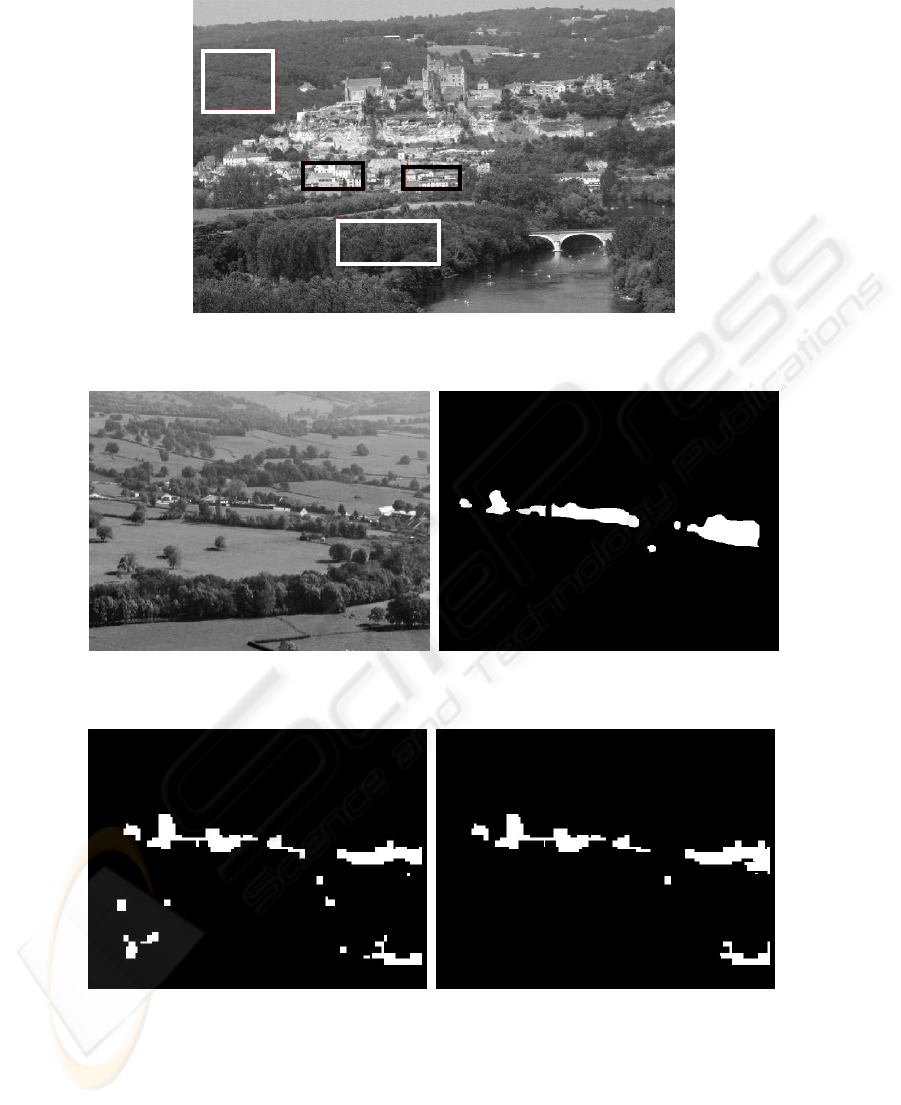
Fig. 1. Learning data base sample. Areas 1 & 2 contain vegetation; areas 3 & 4 contain build-
ings.
Fig. 2. A test image and its ground truth of the test image: white for buildings, black for vege-
tation.
Fig. 3. Buildings recognition without (upper) and with (lower) richness parameter on the left
and right respectively.
1
2
3
4
104

Table 1. Confusion matrix without richness parameter.
Vegetation Buildings
Vegetation 98.6 1.4
Buildings 45.4 54.6
Table 2. Confusion matrix with richness parameter.
Vegetation Buildings
Vegetation 98.6 1.4
Buildings 41.8 58.2
These confusion matrixes are computed pixel per pixel, which is not very favorable to
estimate small object segmentation. So we may notice that:
• 100% of the connected building regions have been detected.
• There is only 1 false alarm (on the bottom right of the image) for building
recognition with the richness parameter.
• Small isolated buildings are still detected when using the richness parameter.
5 Conclusion & Perspectives
We have presented an original idea for texture concept learning using the principle of
fractal compression. This type of learning takes only a few parameters as inputs (per-
centage of texture coverage, number of maximum stored domains) that do not need
any specialist’s skills to be set. Then we have seen a simple recognition step and
some test results. We highlighted the gain of reliability when taking into account the
richness of the classes’ elements used to reconstruct an area. As this is some of our
first test results, the test database size must still be increased to qualify our approach.
Concerning the recognition step, others solutions are available, using for example the
normalized inter correlation to precisely locate similar domains in a straight forward
way.
References
1. Haralick, R.: Statistical and Structural Approaches to Texture, Proc. IEEE, Vol. 67, n°5,
pp. 786-804 (1979).
2. Strzelecki, M.: Segmentation of Textured Biomedical Images Using Neural Networks, PhD
Thesis (1995).
3. Pentland A.: Fractal-Based Description of Natural Scenes, IEEE Trans. Pattern Analysis
and Machine Intelligence, Vol. 6, n°6, pp.661-674 (1984).
4. Kaplan, L., Kuo, C-C.: Texture Roughness Analysis and Synthesis via Extended Self-
similar (ESS) Model, IEEE Trans Pattern Analysis and Machine Intelligence, Vol. 17,
n°11, pp. 1043-1056 (1995).
5. Lepisto, L., Kunttu, I., Autio, J., Visa, A.: Classification method for colored natural tex-
tures using Gabor filtering, Image Analysis and Processing, Proceedings 2003, pp. 397 –
401.
105

6. Ghazel, M., Freeman, G.H., Vrscay, E.R.: Fractal Image Denoising, IEEE Transactions on
Image Processing, Vol. 12, N° 12 (2003).
7. Jacquin, A.: Fractal Image Coding Based on a Theory of Iterated Contractive Image Trans-
formations, Proc. SPIE Visual Comm. And Image Proc., pp. 227-239 (1990).
8. Jacquin, A.: Image Coding Based on a Fractal Theory of Iterated Contractive Image Trans-
formations, IEEE Transactions on Image Processing, Vol. 1, pp. 18-30 (1992).
9. Fisher, Y.: Fractal Image Compression – Theory and Application. New York : Springer-
Verlag (1994).
10. Maria, M.R.J., Benoît, S., Macq, B.: Speeding up fractal image coding by combined DCT
and Kohonen neural net method, ICASSP'98 - IEEE Intl Conference on Acoustics, Speech
and Signal Processing, Proc., pp. 1085-1088 (1998).
11. Vincent, N., Seropian A., Stamon, G.: Synthesis for handwriting analysis, Pattern Recogni-
tion Letters n°26, pp. 267-275 (2004).
12. Chang, H.T.: Gradient Match and Side Match Fractal Vector Quantizers for Images, IEEE
Transactions on image processing, Vol. 11, n°1, January 2002.
13. Lai, Lam, Siu: A fast image coding based on kick-out and zero contrast conditions, IEEE
Transactions on image processing, Vol. 12, n°11 (2003).
14. Hamzaoui, R.: Codebook clustering by self-organizing maps for fractal image compression,
Institut für Informatik – Report 75 (1996).
15. Wohlberg, B.E., De Jager, G.: Fast Image Domain Fractal Compression by DCT Domain
Block Matching, Electronics Letters, Vol. 31, pp. 869-870 (1995).
16. Distasi, R., Nappi, M., Riccio, D.: A Range / Domain Approximation Error-Based Ap-
proach for Fractal Image Compression, IEEE Transactions on Image Processing, Vol. 15,
N° 1, (2006).
17. Barthel, K.U., Schüttemeyer, J., Voyé, T., Noll, P.: A New Image Coding Technique Uni-
fying Fractal and Transform Coding, IEEE International Conference on Image Processing,
(1994).
106
