
UNASSSUMING VIEW-SIZE ESTIMATION TECHNIQUES IN OLAP
An Experimental Comparison
Kamel Aouiche and Daniel Lemire
LICEF, University of Quebec at Montreal, 100 Sherbrooke West, Montreal, Canada
Keywords:
Probabilistic estimation, skewed distributions, sampling, hashing.
Abstract:
Even if storage was infinite, a data warehouse could not materialize all possible views due to the running time
and update requirements. Therefore, it is necessary to estimate quickly, accurately, and reliably the size of
views. Many available techniques make particular statistical assumptions and their error can be quite large.
Unassuming techniques exist, but typically assume we have independent hashing for which there is no known
practical implementation. We adapt an unassuming estimator due to Gibbons and Tirthapura: its theoretical
bounds do not make unpractical assumptions. We compare this technique experimentally with stochastic
probabilistic counting, LOGLOG probabilistic counting, and multifractal statistical models. Our experiments
show that we can reliably and accurately (within 10%, 19 times out 20) estimate view sizes over large data
sets (1.5 GB) within minutes, using almost no memory. However, only GIBBONS-TIRTHAPURA provides
universally tight estimates irrespective of the size of the view. For large views, probabilistic counting has a
small edge in accuracy, whereas the competitive sampling-based method (multifractal) we tested is an order
of magnitude faster but can sometimes provide poor estimates (relative error of 100%). In our tests, LOGLOG
probabilistic counting is not competitive. Experimental validation on the US Census 1990 data set and on the
Transaction Processing Performance (TPC H) data set is provided.
1 INTRODUCTION
View materialization is presumably one of the most
effective technique to improve query performance of
data warehouses. Materialized views are physical
structures that improve data access time by precom-
puting intermediary results. Typical OLAP queries
defined on data warehouses consist in selecting and
aggregating data with queries such as grouping sets
(GROUP BY clauses). By precomputing many plau-
sible groupings, we can avoid aggregates over large
tables. However, materializing views requires addi-
tional storage space and induces maintenance over-
head when refreshing the data warehouse.
One of the most important issues in data ware-
house physical design is to select an appropriate con-
figuration of materialized views. Several heuris-
tics and methodologies were proposed for the ma-
terialized view selection problem, which is NP-
hard (Gupta, 1997). Most of these techniques exploit
cost models to estimate the data access cost using ma-
terialized views, their maintenance and storage cost.
This cost estimation mostly depends on view-size es-
timation.
Several techniques have been proposed for view-
size estimation: some requiring assumptions about
the data distribution and others that are “unassuming.”
A common statistical assumption is uniformity (Gol-
farelli and Rizzi, 1998), but any skew in the data leads
to an overestimate of the size of the view. Generally,
while statistically assuming estimators are computed
quickly, the most expensive step being the random
sampling, their error can be large and it cannot be
bounded a priori.
In this paper, we consider several state-of-the-
art statistically unassuming estimation techniques:
GIBBONS-TIRTHAPURA (Gibbons and Tirthapura,
2001), probabilistic counting (Flajolet and Martin,
1985), and LOGLOG probabilistic counting (Durand
145
Aouiche K. and Lemire D. (2007).
UNASSSUMING VIEW-SIZE ESTIMATION TECHNIQUES IN OLAP - An Experimental Comparison.
In Proceedings of the Ninth International Conference on Enterprise Information Systems - DISI, pages 145-150
DOI: 10.5220/0002354601450150
Copyright
c
SciTePress

and Flajolet, 2003). While relatively expensive, unas-
suming estimators tend to provide a good accuracy.
To our knowledge, this is the first experimental com-
parisons of unassuming view-size estimation tech-
niques in a data warehousing setting.
2 RELATED WORK
Haas et al. (Haas et al., 1995) estimate the view-
size from the histogram of a sample: adaptively, they
choose a different estimator based on the skew of the
distribution. Faloutsos et al. (Faloutsos et al., 1996)
obtain results nearly as accurate as Haas et al., that is,
an error of approximately 40%, but they only need the
dominant mode of the histogram, the number of dis-
tinct elements in the sample, and the total number of
elements. In sample-based estimations, in the worst-
case scenario, the histogram might be as large as the
view size we are trying to estimate. Moreover, it is
difficult to derive unassuming accuracy bounds since
the sample might not be representative. However, a
sample-based algorithm is expected to be an order of
magnitude faster than an algorithm which processes
the entire data set.
Probabilistic counting (Flajolet and Martin, 1985)
and LOGLOG probabilistic counting (henceforth
LOGLOG) (Durand and Flajolet, 2003) have been
shown to provide very accurate unassuming view-size
estimations quickly, but their estimates assume we
have independent hashing. Because of this assump-
tion, their theoretical bound may not hold in practice.
Whether this is a problem in practice is one of the
contribution of this paper.
Gibbons and Tirthapura (Gibbons and Tirtha-
pura, 2001) derived an unassuming bound (henceforth
GIBBONS-TIRTHAPURA) that only requires pairwise
independent hashing. It has been shown recently
that if you have k-wise independent hashing for k >
2 the theoretically bound can be improved substan-
tially (Lemire and Kaser, 2006). The benefit of
GIBBONS-TIRTHAPURA is that as long as the ran-
dom number generator is truly random, the theoret-
ical bounds have to hold irrespective of the size of the
view or of other factors.
All unassuming estimation techniques in this pa-
per (LOGLOG, probabilistic counting and GIBBONS-
TIRTHAPURA), have an accuracy proportional to
1/
√
M where M is a parameter noting the memory
usage.
3 ESTIMATION BY
MULTIFRACTALS
We implemented the statistically assuming algo-
rithm by Faloutsos et al. based on a multifractal
model (Faloutsos et al., 1996). Nadeau and Teo-
rey (Nadeau and Teorey, 2003) reported competitive
results for this approach. Maybe surprisingly, given
a sample, all that is required to learn the multifractal
model is the number of distinct elements in the sam-
ple F
0
, the number of elements in the sample N
0
, the
total number of elements N, and the number of occur-
rences of the most frequent item in the sample m
max
.
Hence, a very simple implementation is possible (see
Algorithm 1). Faloutsos et al. erroneously introduced
a tolerance factor ε in their algorithm: unlike what
they suggest, it is not possible, unfortunately, to ad-
just the model parameter for an arbitrary good fit, but
instead, we have to be content with the best possible
fit (see line 9 and following).
Algorithm 1 View-size estimation using a multifrac-
tal distribution model.
1: INPUT: Fact table t containing N facts
2: INPUT: GROUP BY query on dimensions
D
1
,D
2
,...,D
d
3: INPUT: Sampling ratio 0 < p < 1
4: OUTPUT: Estimated size of GROUP BY query
5: Choose a sample in t
0
of size N
0
= bpNc
6: Compute g=GROUP BY(t
0
)
7: let m
max
be the number of occurrences of the most fre-
quent tuple x
1
,...,x
d
in g
8: let F
0
be the number of tuples in g
9: k ← dlog F
0
e
10: while F < F
0
do
11: p ← (m
max
/N
0
)
1/k
12: F ←
∑
k
a=0
k
a
(1 −(p
k−a
(1 − p)
a
)
N
0
)
13: k ← k + 1
14: p ← (m
max
/N)
1/k
15: RETURN:
∑
k
a=0
k
a
(1 −(p
k−a
(1 − p)
a
)
N
)
4 UNASSUMING VIEW-SIZE
ESTIMATION
4.1 Independent Hashing
Hashing maps objects to values in a nearly random
way. It has been used for efficient data structures such
as hash tables and in cryptography. We are interested
in hashing functions from tuples to [0, 2
L
) where L is
fixed (L = 32 in this paper). Hashing is uniform if
P(h(x) = y) = 1/2
L
for all x, y, that is, if all hashed
ICEIS 2007 - International Conference on Enterprise Information Systems
146

values are equally likely. Hashing is pairwise in-
dependent if P(h(x
1
) = y ∧h(x
2
) = z) = P(h(x
1
) =
y)P(h(x
2
) = z) = 1/4
L
for all x
1
,x
2
,y,z. Pairwise in-
dependence implies uniformity. Hashing is k -wise in-
dependent if P(h(x
1
) = y
1
∧···∧h(x
k
) = y
k
) = 1/2
kL
for all x
i
,y
i
. Finally, hashing is (fully) independent if
it is k-wise independent for all k. It is believed that
independent hashing is unlikely to be possible over
large data sets using a small amount of memory (Du-
rand and Flajolet, 2003).
Next, we show how k-wise independent hashing
is easily achieved in a multidimensional data ware-
housing setting. For each dimension D
i
, we build
a lookup table T
i
, using the attribute values of D
i
as keys. Each time we meet a new key, we gener-
ate a random number in [0, 2L) and store it in the
lookup table T
i
. This random number is the hashed
value of this key. This table generates (fully) inde-
pendent hash values in amortized constant time. In
a data warehousing context, whereas dimensions are
numerous, each dimension will typically have few
distinct values: for example, there are only 8,760
hours in a year. Therefore, the lookup table will of-
ten use a few Mib or less. When hashing a tuple
x
1
,x
2
,.. ., x
k
in D
1
×D
2
×.. .D
k
, we use the value
T
1
(x
1
) ⊕T
2
(x
2
) ⊕···⊕T
k
(x
k
) where ⊕ is the EXCLU-
SIVE OR operator. This hashing is k-wise independent
and requires amortized constant time. Tables T
i
can be
reused for several estimations.
4.2 Probabilistic Counting
Our implementation of (stochastic) probabilistic
counting (Flajolet and Martin, 1985) is given in
Algorithm 2. Recently, a variant of this algo-
rithm, LOGLOG, was proposed (Durand and Flajolet,
2003). Assuming independent hashing, these algo-
rithms have standard error (or the standard deviation
of the error) of 0.78/
√
M and 1.3/
√
M respectively.
These theoretical results assume independent hashing
which we cannot realistically provide. Thus, we do
not expect these theoretical results to be always reli-
able.
4.3 GIBBONS-TIRTHAPURA
Our implementation of the GIBBONS-TIRTHAPURA
algorithm (see Algorithm 4) hashes each tuple only
once unlike the original algorithm (Gibbons and
Tirthapura, 2001). Moreover, the independence of the
hashing depends on the number of dimensions used
by the GROUP BY. If the view-size is smaller than the
memory parameter ( M), the view-size estimation is
Algorithm 2 View-size estimation using (stochastic)
probabilistic counting.
1: INPUT: Fact table t containing N facts
2: INPUT: GROUP BY query on dimensions
D
1
,D
2
,...,D
d
3: INPUT: Memory budget parameter M = 2
k
4: INPUT: Independent hash function h from d tuples to
[0,2
L
).
5: OUTPUT: Estimated size of GROUP BY query
6: b ← M ×L matrix (initialized at zero)
7: for tuple x ∈t do
8: x
0
← π
D
1
,D
2
,...,D
d
(x) {projection of the tuple}
9: y ← h(x
0
) {hash x
0
to [0,2
L
)}
10: α = y mod M
11: i ← position of the first 1-bit in by/Mc
12: b
α,i
← 1
13: A ← 0
14: for α ∈ {0,1,...,M −1} do
15: increment A by the position of the first zero-bit in
b
α,0
,b
α,1
,...
16: RETURN: M/φ2
A/M
where φ ≈ 0.77351
Algorithm 3 View-size estimation using LOGLOG.
1: INPUT: fact table t containing N facts
2: INPUT: GROUP BY query on dimensions
D
1
,D
2
,...,D
d
3: INPUT: Memory budget parameter M = 2
k
4: INPUT: Independent hash function h from d tuples to
[0,2
L
).
5: OUTPUT: Estimated size of GROUP BY query
6: M ← 0, 0, . . . , 0
| {z }
M
7: for tuple x ∈t do
8: x
0
← π
D
1
,D
2
,...,D
d
(x) {projection of the tuple}
9: y ← h(x
0
) {hash x
0
to [0,2
L
)}
10: j ← value of the first k bits of y in base 2
11: z ← position of the first 1-bit in the remaining L −k
bits of y (count starts at 1)
12: M
j
← max(M
j
,z)
13: RETURN: α
M
M2
1
M
∑
j
M
j
where α
M
≈ 0.39701 −
(2π
2
+ ln
2
2)/(48M).
without error. For this reason, we expect GIBBONS-
TIRTHAPURA to perform well when estimating small
and moderate view sizes.
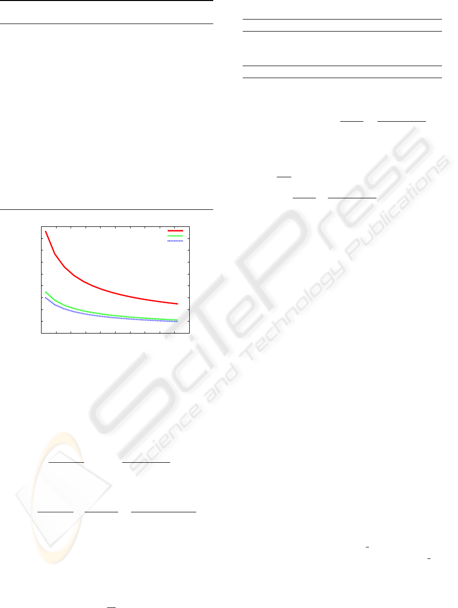
The theoretical bounds given in (Gibbons and
Tirthapura, 2001) assumed pairwise independence.
The generalization below is from (Lemire and Kaser,
2006) and is illustrated by Figure 1.
Proposition 1 Algorithm 4 estimates the number of
distinct tuples within relative precision ε, with a k-
wise independent hash for k ≥ 2 by storing M distinct
tuples (M ≥ 8k) and with reliability 1 −δ where δ is
UNASSSUMING VIEW-SIZE ESTIMATION TECHNIQUES IN OLAP - An Experimental Comparison
147
Algorithm 4 GIBBONS-TIRTHAPURA view-size esti-
mation.
1: INPUT: Fact table t containing N facts
2: INPUT: GROUP BY query on dimensions
D
1
,D
2
,...,D
d
3: INPUT: Memory budget parameter M
4: INPUT: k-wise hash function h from d tuples to [0,2
L
).
5: OUTPUT: Estimated size of GROUP BY query
6: M ← empty lookup table
7: t ←0
8: for tuple x ∈t do
9: x
0
← π
D
1
,D
2
,...,D
d
(x) {projection of the tuple}
10: y ← h(x
0
) {hash x
0
to [0,2
L
)}
11: j ← position of the first 1-bit i y (count starts at 0)
12: if j ≤t then
13: M
x
0
= j
14: while size(M ) > M do
15: t ←t + 1
16: prune all entries in M having value less than t
17: RETURN:.2
t
size(M )
0
0.1
0.2
0.3
0.4
0.5
0.6
0.7
0.8
0.9
200 400 600 800 1000 1200 1400 1600 1800 2000 2200
ε 19/20
M
k=2
k=4
k=8
Figure 1: Bound on the estimation error (19 times out of
20) as a function of the number of tuples kept in memory
(M ∈[128, 2048]) according to Proposition 1 for GIBBONS-
TIRTHAPURA view-size estimation with k -wise indepen-
dent hashing.
given by
δ =
k
k/2
e
k/3
M
k/2
2
k/2
+
8
k/2
ε
k
(2
k/2
−1)
!
.
More generally, we have
δ ≤
k
k/2
e
k/3
M
k/2
α
k/2
(1 −α)
k
+
4
k/2
α
k/2
ε
k
(2
k/2
−1)
!
.
for 4k/M ≤ α < 1 and any k,M > 0.
In the case where hashing is 4-wise independent,
as in some of experiments below, we derive a more
concise bound.
Corollary 1 With 4-wise independent hashing, Algo-
rithm 4 estimates the number of distinct tuples within
relative precision ε ≈ 5/
√
M, 19 times out of 20 for ε
small.
Table 1: Characteristic of data sets.
US Census 1990 DBGEN
# of facts 2458285 13977981
# of views 20 8
# of attributes 69 16
Data size 360 MB 1.5 GB
Proof. We start from the second inequality of Propo-
sition 1. Differentiating
α
k/2
(1−α)
k
+
4
k/2
α
k/2
ε
k
(2
k/2
−1)
with
respect to α and setting the result to zero, we get
3α
4
ε
4
+ 16α
3
−48α
2
−16 = 0 (recall that 4k/M ≤
α < 1). By multiscale analysis, we seek a solution of
the form α = 1 −aε
r
+ o(ε
r
) and we have that α ≈
1 −1/2
3
p
3/2ε
4/3
for ε small. Substituting this value
of α, we have
α
k/2
(1−α)
k
+
4
k/2
α
k/2
ε
k
(2
k/2
−1)
≈128/24ε
4
. The
result follows by substituting in the second inequal-
ity.
5 EXPERIMENTAL RESULTS
To benchmark the quality of the view-size estima-
tion against the memory and speed, we have run test
over the US Census 1990 data set (Hettich and Bay,
2000) as well as on synthetic data produced by DB-
GEN (TPC, 2006). The synthetic data was produced
by running the DBGEN application with scale factor
parameter equal to 2. The characteristics of data sets
are detailed in Table 1. We selected 20 and 8 views re-
spectively from these data sets: all views in US Cen-
sus 1990 have at least 4 dimensions whereas only 2
views have at least 4 dimensions in the synthetic data
set.
We used the GNU C++ compiler version 4.0.2
with the “-O2” optimization flag on a Centrino Duo
1.83 GHz machine with 2 GB of RAM running Linux
kernel 2.6.13–15. No thrashing was observed. To
ensure reproducibility, C++ source code is available
freely from the authors.
For the US Census 1990 data set, the hashing
look-up table is a simple array since there are always
fewer than 100 attribute values per dimension. Oth-
erwise, for the synthetic DBGEN data, we used the
GNU/CGI STL extension hash map which is to be
integrated in the C++ standard as an unordered map:
it provides amortized O(1) inserts and queries. All
other look-up tables are implemented using the STL
map template which has the same performance char-
acteristics of a red-black tree. We used comma sep-
arated (CSV) (and pipe separated files for DBGEN)
text files and wrote our own C++ parsing code.
ICEIS 2007 - International Conference on Enterprise Information Systems
148

The test protocol we adopted (see Algorithm 5)
has been executed for each estimation technique
(LOGLOG, probabilistic counting and GIBBONS-
TIRTHAPURA), GROUP BY query, random seed and
memory size. At each step corresponding to those pa-
rameter values, we compute the estimated-size values
of GROUP BY s and time required for their compu-
tation. For the multifractal estimation technique, we
computed at the same way the time and estimated size
for each GROUP BY, sampling ratio value and ran-
dom seed.
Algorithm 5 Test protocol.
1: for GROUP BY query q ∈ Q do
2: for memory budget m ∈ M do
3: for random seed value r ∈ R do
4: Estimate the size of GROUP BY q with m mem-
ory budget and r random seed value
5: Save estimation results (time and estimated
size) in a log file
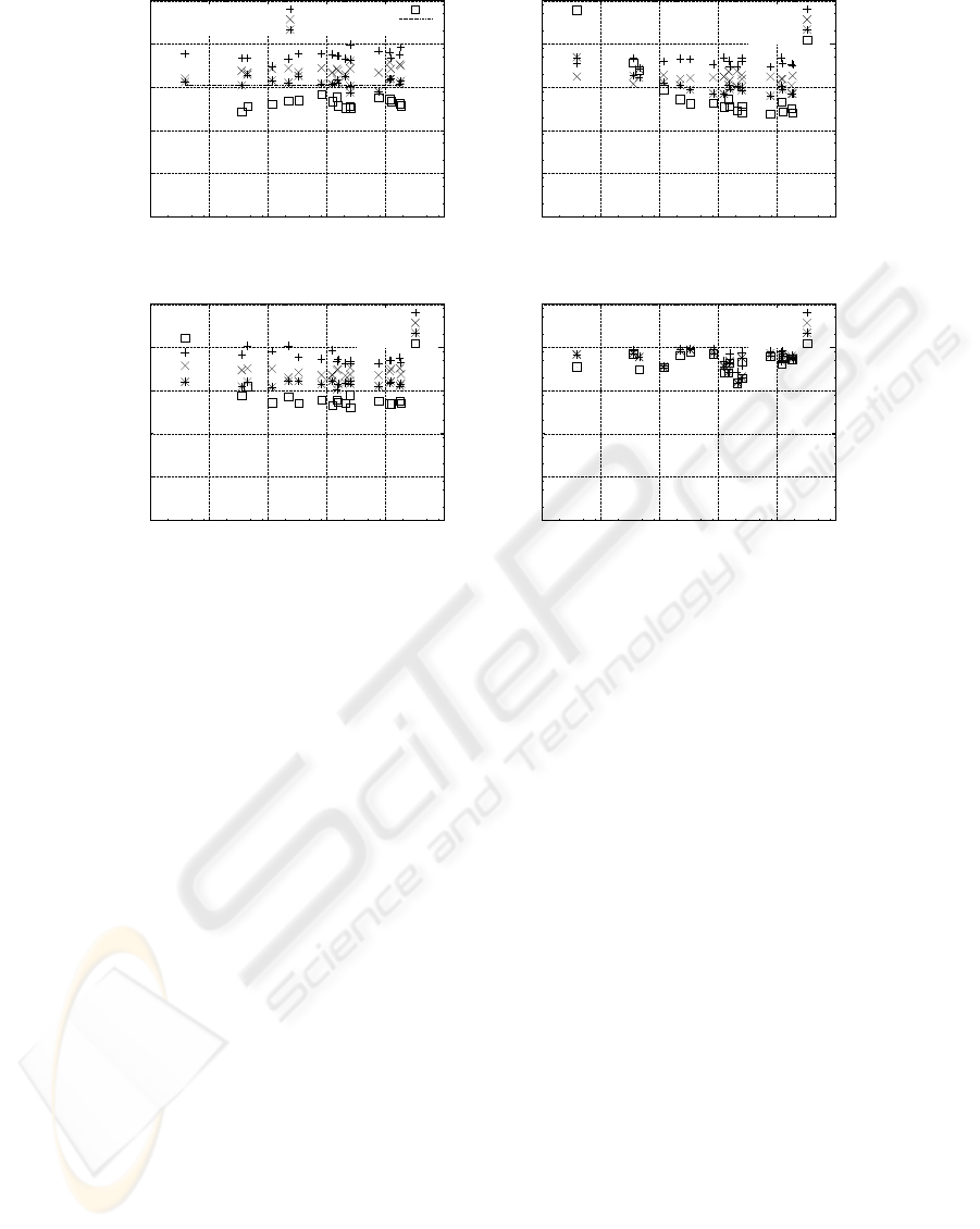
US Census 1990. Figure 2 plots the largest 95
th
-
percentile error observed over 20 test estimations
for various memory size M ∈ {16, 64,256, 2048}.
For the multifractal estimation technique, we rep-
resent the error for each sampling ratio p ∈
{0.1%,0.3%,0.5%, 0.7%}. The X axis represents
the size of the exact GROUP BY values. This
95
th
-percentile error can be related to the theoreti-
cal bound for ε with 19/20 reliability for GIBBONS-
TIRTHAPURA (see Corollary 1): we see that this up-
per bound is verified experimentally. However, the er-
ror on “small” view sizes can exceed 100% for prob-
abilistic counting and LOGLOG.
Synthetic data set. Similarly, we computed the
19/20 error for each technique, computed from the
DDBGEN data set . We observed that the four tech-
niques have the same behaviour observed on the US
Census data set. Only, this time, the theoretical bound
for the 19/20 error is larger because the synthetic data
sets has many views with less than 2 dimensions.
Speed. We have also computed the time needed for
each technique to estimate view-sizes. We do not rep-
resent this time because it is similar for each tech-
nique except for the multifractal which is the fastest
one. In addition, we observed that time do not depend
on the memory budget because most time is spent
streaming and hashing the data. For the multifrac-
tal technique, the processing time increases with the
sampling ratio.
The time needed to estimate the size of all
the views by GIBBONS-TIRTHAPURA, probabilis-
tic counting and LOGLOG is about 5 minutes for
US Census 1990 data set and 7 minutes for the syn-
thetic data set. For the multifractal technique, all
the estimates are done on roughly 2 seconds. This
time does not include the time needed for sampling
data which can be significant: it takes 1 minute (resp.
4 minutes) to sample 0.5% of the US Census data set
(resp. the synthetic data set – TPC H) because the
data is not stored in a flat file.
6 DISCUSSION
Our results show that probabilistic counting and
LOGLOG do not entirely live up to their theoretical
promise. For small view sizes, the relative accuracy
can be very low.
When comparing the memory usage of the var-
ious techniques, we have to keep in mind that the
memory parameter M can translate in different mem-
ory usage. The memory usage depends also on
the number of dimensions of each view. Generally,
GIBBONS-TIRTHAPURA will use more memory for
the same value of M than either probabilistic counting
or LOGLOG, though all of these can be small com-
pared to the memory usage of the lookup tables T
i
used for k-wise independent hashing. In this paper,
the memory usage was always of the order of a few
MiB which is negligible in a data warehousing con-
text.
View-size estimation by sampling can take min-
utes when data is not layed out in a flat file or in-
dexed, but the time required for an unassuming es-
timation is even higher. Streaming and hashing the
tuples accounts for most of the processing time so for
faster estimates, we could store all hashed values in a
bitmap (one per dimension).
7 CONCLUSION AND FUTURE
WORK
In this paper, we have provided unassuming tech-
niques for view-size estimation in a data warehousing
context. We adapted an estimator due to Gibbons and
Tirthapura. We compared this technique experimen-
tally with stochastic probabilistic counting, LOGLOG,
and multifractal statistical models. We have demon-
strated that among these techniques, only GIBBONS-
TIRTHAPURA provides stable estimates irrespective
of the size of views. Otherwise, (stochastic) proba-
bilistic counting has a small edge in accuracy for rela-
tively large views, whereas the competitive sampling-
based technique (multifractal) is an order of mag-
nitude faster but can provide crude estimates. Ac-
cording to our experiments, LOGLOG was not faster
UNASSSUMING VIEW-SIZE ESTIMATION TECHNIQUES IN OLAP - An Experimental Comparison
149
0.01
0.1
1
10
100
1000
100 1000 10000 100000 1e+006 1e+007
ε(%), 19 out of 20
View size
M=16
M=64
M=256
M=2048
4-wise M=2048
(a) GIBBONS-TIRTHAPURA
0.01
0.1
1
10
100
1000
100 1000 10000 100000 1e+06 1e+07
ε(%), 19 out of 20
View size
M=16
M=64
M=256
M=2048
(b) Probabilistic counting
0.01
0.1
1
10
100
1000
100 1000 10000 100000 1e+06 1e+07
ε(%), 19 out of 20
View size
M=16
M=64
M=256
M=2048
(c) LOGLOG
0.01
0.1
1
10
100
1000
100 1000 10000 100000 1e+06 1e+07
ε(%), 19 out of 20
View size
p=0.1%
p=0.3%
p=0.5%
p=0.7%
(d) Multifractal
Figure 2: 95
th
-percentile error 19/20 ε as a function of exact view size for increasing values of M (US Census 1990).
than either GIBBONS-TIRTHAPURA or probabilistic
counting, and since it is less accurate than probabilis-
tic counting, we cannot recommend it. There is ample
room for future work. Firstly, we plan to extend these
techniques to other types of aggregated views (for ex-
ample, views including HAVING clauses). Secondly,
we want to precompute the hashed values for very
fast view-size estimation. Furthermore, these tech-
niques should be tested in a materialized view selec-
tion heuristic.
ACKNOWLEDGEMENTS
The authors wish to thank Owen Kaser for hardware
and software. This work is supported by NSERC
grant 261437 and by FQRNT grant 112381.
REFERENCES
Durand, M. and Flajolet, P. (2003). Loglog counting of
large cardinalities. In ESA’03. Springer.
Faloutsos, C., Matias, Y., and Silberschatz, A. (1996). Mod-
eling skewed distribution using multifractals and the
80-20 law. In VLDB’96, pages 307–317.
Flajolet, P. and Martin, G. (1985). Probabilistic counting al-
gorithms for data base applications. Journal of Com-
puter and System Sciences, 31(2):182–209.
Gibbons, P. B. and Tirthapura, S. (2001). Estimating simple
functions on the union of data streams. In SPAA’01,
pages 281–291.
Golfarelli, M. and Rizzi, S. (1998). A methodological
framework for data warehouse design. In DOLAP
1998, pages 3–9.
Gupta, H. (1997). Selection of views to materialize in a data
warehouse. In ICDT 1997, pages 98–112.
Haas, P., Naughton, J., Seshadri, S., and Stokes, L. (1995).
Sampling-based estimation of the number of distinct
values of an attribute. In VLDB’95, pages 311–322.
Hettich, S. and Bay, S. D. (2000). The UCI KDD
archive. http://kdd.ics.uci.edu, last checked on
32/10/2006.
Lemire, D. and Kaser, O. (2006). One-pass, one-hash
n-gram count estimation. Technical Report TR-06-
001, Dept. of CSAS, UNBSJ. available from http:
//arxiv.org/abs/cs.DB/0610010.
Nadeau, T. and Teorey, T. (2003). A Pareto model for OLAP
view size estimation. Information Systems Frontiers,
5(2):137–147.
TPC (2006). DBGEN 2.4.0. http://www.tpc.org/
tpch/, last checked on 32/10/2006.
ICEIS 2007 - International Conference on Enterprise Information Systems
150
