
CUSTOMER BEHAVIOR MODELING UNDER SEVERAL
DECISION-MAKING PROCESSES BY USING EM ALGORITHM
Takeshi Kurosawa, Ken Nishimatsu, Motoi Iwashita
NTT Service Integration Laboratories, 3-9-11 Midori-Cho, Musashino, Tokyo, Japan
Akiya Inoue
Department of Management Information Science, Chiba Institute of Technology,2-17-1 Tsudanuma,Narashino ,Chiba, Japan
Keywords:
Discrete Choice Analysis, EM-Algorithm, Decision Making Process, Consumer Behavior, Data and Knowl-
edge Engineering.
Abstract:
This paper gives a model of customer choice behavior modeling based on a combination of decision-making
processes by applying latent class model based on EM algorithm. This model can apply for the choice prob-
lems of multi services and multi brands under various decision-making processes. In addition to the model
based on EM algorithm, we tried some conventional models and compared them. The model based on EM
algorithm enables us to know what kinds of customers are classified into a certain class. Moreover, we could
construct more accuracy model than conventional model and found the existence of two decision-making
processes.
1 INTRODUCTION
The amount of the traffic flowing in the network de-
pends on the number of customers. Therefore the
estimation of the number of customers is very im-
portant factor in the network design. Generally cus-
tomer choice behavior modeling is very complicated.
These days, customers are faced with a wide range of
choice for telecommunications services. This arises
from the rapid progress of information and communi-
cation technology and the competitive environment.
Therefore, customers use various different decision-
making processes to select a service that provides
the features they want. Here, the decision-making
process means the order of selection when the cus-
tomer chooses the service. However, we generally
cannot know what kind of decision-making process
they are using. In such a situation, we cannot fully
express customer choice behavior by using model
whose structure is based on a single decision-making
process. Therefore, a model that takes into consider-
ation a customer’s complicated decision-making pro-
cesses is needed. Main purpose of this paper is to
give customer choice behavior modeling under sev-
eral decision-making processes because the accuracy
of the customer choice behavior modeling gives us
more accuracy traffic estimation and service demand
estimation.
For this purpose, we use a latent class model using
the EM algorithm. We regard a decision-making pro-
cess as one latent class of EM algorithm. One class
model is expressed by the hierarchy structure. In this
paper, we explain our model and present results that
verify it.
2 RELATED WORK
The telephone service market is fiercely competitive.
Both the telephone service and Internet service mar-
kets are changing rapidly as technology progresses.
Therefore, it is not always appropriate to forecast ser-
vice demand by using conventional time series anal-
ysis based on measurement data obtained in network
management systems. Some researchers have studied
markets such as Internet service (Savage and Wald-
man, 2004; Loomis and Taylor, 2001) and telephone
services (Fildes and Kumar, 2002; Loomis and Tay-
lor, 1999). These described to only one service model.
We have proposed the technique of Scenario Sim-
ulation (Inoue et al., 2003a; Inoue et al., 2003b;
Nishimatsu et al., 2004; Takahashi et al., 2004; Nishi-
339
Kurosawa T., Nishimatsu K., Iwashita M. and Inoue A. (2007).
CUSTOMER BEHAVIOR MODELING UNDER SEVERAL DECISION-MAKING PROCESSES BY USING EM ALGORITHM.
In Proceedings of the Second International Conference on e-Business, pages 339-346
DOI: 10.5220/0002115703390346
Copyright
c
SciTePress

matsu et al., 2005; Nishimatsu et al., 2006), which
uses customer choice behavior modeling. This mod-
eling (See the appendix A.1) is used to estimate the
demand for a service and the amount of traffic that
will flow through the network. Therefore, enhancing
the accuracy of customer choice behavior modeling is
the most important factor in Scenario Simulation.
Usually, we use Discrete Choice Analysis (Ben-
Akiva and Lerman, 1985; Train, 2003)(DCA) to con-
struct a customer choice behavior model. DCA (See
the appendix A.2) is the technique derived from the
field of traffic engineering and it is applied in vari-
ous fields. Customer choice behavior modeling for
a telecommunications service has been analyzed us-
ing DCA (Kurosawa et al., 2005; Kurosawa et al.,
2006). One reason for the complexity of the tele-
phone market is that a customer can get the features
he/she wants by combining multiple services. For ex-
ample, a customer who wants to use IP telephony may
make separate contracts with an Internet access line
provider, an Internet service provider (ISP), and an IP
telephony provider. This combination of services can
more economical for Internet users than using POTS
(plain old telephone service). A nested structure can
express the priority or the order of selecting. We can
consider the priority or the order of selecting as a
decision-making process. To solve the problem, cus-
tomer choice behavior modeling using a nested struc-
ture was examined (Kurosawa et al., 2006). That ex-
amination showed the existence of a decision-making
process with a nested structure. The paper concluded
that one decision-making process is more appropri-
ate than other models. The research (Ben-Akiva and
Gershenfeld, 1998) focused on the combination of op-
tional services. However, customers do not always all
use the same decision-making process. Namely, two
or more decision-making processes may exist. How-
ever, we cannot know which decision-making process
a given customer will use. To handle this characteris-
tic, we focused on the EM algorithm. This algorithm
complements imperfect data by using expected val-
ues obtained through the application of Bayes’ the-
ory. That is, posterior probability is used as the ex-
pected value. This framework is used for the latent
class model. Generally, we cannot know which kind
of latent class the customer belongs to. So the EM al-
gorithm obtains the probability of belonging to a class
by using an expected value.
In this case study, we verified the accuracy of our
model. And we focused on what kinds of customers
are classified into a certain class (decision-making
process) because the class model has individual vari-
ables.
3 CHOICE MODEL UNDER
VARIOUS DECISION-MAKING
PROCESSES
We use DCA models in each step of the EM al-
gorithm. There are two types of model. As-
sume that S decision-making processes exist. There-
fore, we consider S decision-making process models
P
1
(i|C;β
1
;x),. ..,P
S
(i|C;β
S
;x). These models repre-
sent the probability of service i being chosen from the
universal choice set C under decision-making process
s (s = 1,...,S). Here, x and β
s
are an explanatory
variable vector and a coefficient vector, respectively.
Suppose that the number of elements in the universal
choice set C is G. That is, there are G combination
of the services in the market. One decision-making
process corresponds to one nested logit (NL) model
(Ben-Akiva and Lerman, 1985; Train, 2003) which
is a type of DCA model. This model can capture
one decision-making process. This is explained in de-
tail in section 3.2. The other model is a class model
π(s;γ;x), where x and γ are the explanatory variable
vector and the coefficient vector, respectively. This
model gives the probability that a customer belongs to
certain decision-making process (class). In this way,
we get the probability of service i being chosen from
universal choice set C as
P(i|C;γ,β;x) =
S
∑
s=1
π(s;γ;x)P
s
(i|C;β
s
;x). (1)
The structure of our model is shown in Fig. 1. This
figure assumes that there are three types of decision-
making processes.
Figure 1: Choice Model under Various Decision-Making
Processes.
3.1 Class Model
In this section, we define a class model π(s;γ;x) (0 ≤
π(s;γ;x) ≤ 1 and
∑
S
s=1
π(s;γ;x) = 1) by using MNL
in DCA (See the appendix A.2). The probability
π
n
(s;γ) of customer n using decision-making process
s is given by
π
n
(s;γ) = π(s;γ;x
n
), (2)
ICE-B 2007 - International Conference on e-Business
340

where x
n
mean attribute values of customer n.
We need the systematic term of utility functions
R
1n
,.. . ,R
Sn
(corresponding to V
in
in the appendix
A.2). By using these utility functions, we get
π
n
(s;γ) =
exp(µR
sn
)
∑
S
j=1
exp(µR
jn
)
. (3)
Since R
sn
include individual attributes, we can deter-
mine what kind of customers belong to what kind of
decision-making process.
3.2 Decision-Making Process
This section shows how to construct decision-making
process models. We use customer choice results to
construct them. That is, customer n chooses a service
from choice set C
tn
, t (1 ≤ t ≤ T
n
) times. Then, we
defined these explanatory data as x
tn
(t = 1, ... , T
n
).
Here, the probability P
stn
(i|C
tn
;β
s
) of service i being
chosen by customer n through decision-making pro-
cess s is defined as
P
stn
(i|C
tn
;β
s
) = P
s
(i|C;β
s
;x
tn
). (4)
To express a decision-making process, we need a hier-
archal structure like a decision tree because a decision
tree can capture the selection order and the correlation
among alternatives. Since this NL model has a hierar-
chical structure representing the decision-making pro-
cess, it is possible to express the model according to
the sequence of selections. Let D
s
be the depth of the
layered structure. A decision-making structure with a
depth of 2 is shown in Fig. 2 as an example.
Figure 2: Nested logit model (depth=2).
A structure with a depth of 3 is shown in Fig. 3.
The service i is included in a certain alternative
subsets sequence i ∈ C
(1)
m
1
stn
⊂ ··· ⊂ C
(D
s
−1)
m
D
s
−1
stn
⊂ C
tn
.
The systematic terms of utility function V
(d)
k
d
stn
of
C
(d)
k
d
stn
(1 ≤ k
d
≤ M
d
) is defined. For example, as seen
in Fig. 2, when the depth of the decision-making
structure is 2 level hierarchy and the error term is
EV1, the probability of subset C
(1)
m
1
stn
being chosen
from all alternative sets C
tn
is given by
P
stn
(C
(1)
m
1
stn
|C
tn
) =
exp(µ
s
V
(1)
m
1
stn
)
∑
k
1
=1,...,M
1
exp(µ
s
V
(1)
k
1
stn
)
, (5)
Figure 3: Nested logit model (depth=3).
whereV
(1)
k
1
stn
=
1
µ
sk
1
ln
∑
i∈C
(1)
k
1
stn
exp(µ
sk
1
V
(2)
istn
) (1 ≤ k
1
≤
M
1
). Here, the nesting coefficients µ
s
and µ
sk
1
are unknown parameters which are greater than 0.
These nesting coefficients represent the relationship
between a high-level nest and a low-level nest. It is
desirable for the relationship between the nesting co-
efficient and the top nesting coefficient µ
s
to be like
1 = µ
s
≤ µ
sk
1
, (6)
for 1 ≤ k
1
≤ M
1
). Generally, it is required that 1 =
µ
s
≤ µ
sk
1
≤ ··· ≤ µ
sk
1
···k
D
s
−1
(1 ≤ k
d
≤ M
d
,1 ≤ d ≤
D
s
− 1). At the second layer, the probability that al-
ternative i is chosen from subset C
(1)
m
1
stn
is given by
P
stn
(i|C
(1)
m
1
stn
) =
exp(µ
sm
1
V
(2)
istn
)
∑
j∈C
(1)
m
1
stn
exp(µ
sm
1
V
(2)
jstn
)
. (7)
Therefore, the probability that alternative i is chosen
from all alternative sets C
tn
is expressed as
P
stn
(i|C
tn
;β
s
) = P
stn
(i|C
(1)
m
1
stn
)P
stn
(C
(1)
m
1
stn
|C
tn
), (8)
where β
s
is an unknown parameter vector that appears
in all utility functions in the decision-making process
s. All nesting coefficients are also contained in un-
known parameter vector β
s
. Moreover, equation (8) is
generalized to
P
stn
(i|C
tn
;β
s
) = P
stn
(i|C
(1)
m
1
stn
)
×
D
s
−2
∏
d=1
P
stn
(C
(d)
m
d
stn
|C
(d+1)
m
d+1
stn
)
!
P
stn
(C
(D
s
−1)
m
D
s
−1
stn
|C
tn
).
(9)
In this way, we can substitute (8) or (9) into (4).
3.3 Likelihood Function
We can get π
n
(s;γ) and P
stn
(i|C
tn
;β
s
) from (3) and (9),
respectively. Therefore, after determining the follow-
ing probability
P
tn
(i|C
tn
;γ,β) =
∑
S
s=1
π
n
(s;γ)P
stn
(i|C
tn
;β
s
), (10)
CUSTOMER BEHAVIOR MODELING UNDER SEVERAL DECISION-MAKING PROCESSES BY USING EM
ALGORITHM
341

we can get equation (1) by using (2) and (4). Then,
the maximum likelihood function is defined by
L(γ,β;y, z) =
N
∏
n=1
S
∏
s=1
( f
sn
(y
n
;β
s
)π
n
(s;γ))
z
ns
, (11)
where
f
sn
(y
n
;β
s
) =
T
n
∏
t=1
∏
i∈C
tn
P
stn
(i|C
tn
;β
s
)
y
tn
(i)
.
Here, z
ns
is a dummy variable that takes the value 1
or 0. It is 1 when customer n belongs to a given class
s and 0 when he/she does not. This value is not an
observable variable because we cannot know which
kind of decision-making process a customer will use
to choose a service. Hence, we solve this problem by
using the EM algorithm method. The probability of
belonging to this class (decision-making process) is
given in section 3.4.
3.4 E-Step
Since we do not know what kind of decision-making
process a customer uses when he/she selects a service,
we replace z
ns
by an expectation value obtained using
Bayes’ theory in this E-step (expectation-step). The
posterior probability Q
n
(s) is defined by
Q
n
(s) =
π
n
(s;γ) f
sn
(y
n
;β
s
)
S
∑
j=1
π
n
( j;γ) f
jn
(y
n
;β
j
)
. (12)
Namely, π
n
( j;γ) is given as a prior probability while
Q
n
(s) is given as a posterior probability. In the first
step, since γ and β are unknown parameter vectors,
Q
n
(s), which is randomly assigned a value between 0
an 1 since it is a probability, is given to every user n.
Hence, by replacing z
ns
by E
z
[z
ns
] = Q
n
(s), we get the
likelihood function as
E
z
[logL(γ,β;y,z)]
=
N
∑
n=1
S
∑
s=1
Q
n
(s)log f
sn
(y
n
;β
s
)
+
N
∑
n=1
S
∑
s=1
Q
n
(s)logπ
n
(s;γ)
=
S
∑
s=1
N
∑
n=1
T
n
∑
t=1
Q
n
(s)log
∏
i∈C
n
P
stn
(i|C
tn
;β
s
)
y
tn
(i)
!
+
N
∑
n=1
S
∑
s=1
Q
n
(s)logπ
n
(s;γ)
=
∑
S
s=1
L
s
(β
s
) +
L
∗
(γ). (13)
3.5 M-Step
For given log-likelihood function (13), we find val-
ues of γ and β that maximize it. From equation (13),
the log-likelihood function is composed of S+ 1 log-
likelihood functions. Since unknown parameters in
γ and β are separated for each log-likelihood func-
tion, we may maximize these S + 1 log-likelihood
functions independently. In this way, we find the
maximum solution of the log-likelihood function
E
z
[logL(γ,β;y,z)]. Let
ˆ
β and
ˆ
γ be the maximum solu-
tions of the log-likelihood function. When we substi-
tuting the obtained
ˆ
β and
ˆ
γ into (12), the flow returns
to the E-step. In this way, the E-step and M-step are
executed repeatedly until the log-likelihood function
converges.
4 CASE STUDY
4.1 Menu and Sample
To verify our model, we tested the model with choice
data. We used an online questionnaire system to col-
lect choice data, which were related to the choice
of telephone company. In February 2005, we asked
people which company they would choose and what
kind of optional telephone services they would like
to use The choices included some basic service at-
tributes such as the monthly telephone service charge,
the charge for local calls, and five optional services
such as a multiple number service. Optional ser-
vice charges were presented for each company, and
optional services could be selected independently of
company choice. Moreover, the choices included two
kinds of discounts (Bundle 1 and 2) for combined op-
tional services. There were four representative com-
panies (Companies A, B, C, and D) and five optional
services (OP1, .. . , OP5). We classified the types of
optional services as follows.
Type 1 No optional services included
Type 2 Non bundling with at least one optional ser-
vice included
Type 3 Bundle 1 discount included
Type 4 Bundle 2 discount included
Type 5 Bundle 1 and 2 discounts included
Thus, there were 4 brands and 5 types of optional ser-
vice. That is, a customer had a choice of 4× 5 + 1 =
21 different alternatives. Here, +1 means not using
any telephone service. This alternative was named 50.
For example, alternative 31 means company C (brand
3) and option type 1 (see Fig. 4). Our questionnaire
ICE-B 2007 - International Conference on e-Business
342
survey received responses from N = 3450 people. Be-
cause they answered the questionnaire 2 or 3 times for
different conditions, we got
∑
N
n=1
T
n
= 7971 observa-
tions. Table 1 shows how many users selected each
brand and option type. ‘None’ means that the cus-
tomer doesn’t select a telephone service.
Table 1: Customer choice distribution.
Brand1 2 3 4 Sum
Type1 666 399 232 122 1419
Type2 1000 592 417 223 2232
Type3 98 60 31 27 216
Type4 1318 748 527 271 2864
Type5 435 253 174 109 971
Sum 3517 2052 1381 752 7702
None - - - - 269
7971
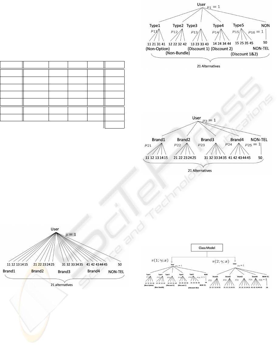
4.2 Implementation
We performed three types of modeling: MNL, NL,
and our EM-algorithm-based model. NL captures a
decision-making process such as a sequence of choos-
ing alternatives and a choice criterion by expressing a
hierarchical structure. In our case study, we simulated
two kinds of NL models. Therefore, we regarded the
total number of models as being 4.
1. MNL model
Figure 4: MNL model.
In the MNL model, the alternatives are at the same
level in the hierarchy. That is, there are 21 alter-
natives at the same level (see Fig. 4).
2. NL model 1: choosing optional services first
In this choice model, we assume that a customer
chooses an optional service type at level 1 in Fig.
5. Finally, the customer compares companies. We
call this model NL1. The key feature of this model
is the nodes for the six types.
Figure 5: NL model 1.
3. NL model 2: choosing a company first
Figure 6: NL model 2.
In this choice model, we assume that a customer
chooses a company at level 1 and then chooses
the type of optional services at level 2. We call
this model NL2.
4. Model based on the EM algorithm
Figure 7: Model based on the EM algorithm.
This model is based on the EM algorithm. There
are two decision-making processes, that is, this
model includes the two above-mentioned nested
logit models NL1 and NL2.
We used BIOGEME to estimate the MNL, NL1, and
NL2 models. This software is an estimator devel-
oped for DCA models(Bierlaire, 2005). It is splen-
did software for analyzing DCA models. Moreover,
we implemented EM algorithm software to verify our
CUSTOMER BEHAVIOR MODELING UNDER SEVERAL DECISION-MAKING PROCESSES BY USING EM
ALGORITHM
343

model. This EM algorithm software uses BIOGEME
as a core engine for estimation.
4.3 Results
The simulation results for the four models are briefly
presented below. We mainly used adjusted rho
squared
ρ
2
to show the validity of each model (see
the appendix A.2) and nesting coefficients µ.
4.3.1 Results for MNL Model
In the MNL model, we estimated all 21 alternatives
simultaneously. Table 2 shows some of the estima-
tion results obtained with the MNL model. Here,
Table 2: Results for MNL model.
Value t-value Robust t-value
b Bundle1 -42.956 -50.41 -53.51
b Bundle2 -13.403 -51.81 -46.98
b OP1Ch -2.4219 -15.50 -12.63
b OP2Ch -4.6167 -10.45 -9.13
b OP3Ch -5.8008 -15.56 -11.08
b OP4Ch -4.8205 -21.69 -16.95
b OP5Ch -1.6230 -5.51 -4.44
b monthCh -3.5199 -44.31 -38.22
b Bundle1Ch and b Bundle2Ch mean the discount
for bundling optional services. b
OP1Ch and so on
are the charges for optional services, and b
monthCh
is the monthly charge for telephone service. All co-
efficients of explanatory variables have good signs,
where a good sign means, for example, that the utility
goes down in value when the monthly charge goes up.
Moreover, these coefficients have high t-values.
4.3.2 Results for NL Models
NL1 and NL2 obtained good signs, the same as those
in Table 2 for the MNL model. The difference be-
tween the MNL model and the NL models is the nest-
ing coefficient. Tables 3 and 4 show estimated nesting
coefficients.
Table 3: Nesting coeffi-
cients of NL1.
Name Value
µ
11
1.0000
µ
12
1.0000
µ
13
1.0000
µ
14
1.0000
µ
15
1.0000
µ
16
1 (Fix)
Table 4: Nesting coeffi-
cients of NL2.
Name Value
µ
21
6.1707
µ
22
6.9078
µ
23
5.9584
µ
24
6.5349
µ
25
1 (Fix)
The nesting coefficients of NL1 were estimated
to be 1 in Table 3. By the equation (6), we can see
that µ
1
= µ
1k
1
(1 ≤ k
1
≤ 6). This means NL1 model
does not have the nodes in Fig. 5. That is, the NL1
model is regarded as the MNL model. We can also
see evidence of this in Table 9 because the
ρ
2
of
NL1 and MNL are nearly equal. On the other hand,
µ
2k
1
(1 ≤ k
1
≤ 5) are greater than 1. This means the
NL2 has the nesting structure. NL1 and NL2 have in
inverse relationship, so these results are not strange.
Namely, NL2 is more appropriate than NL1.
4.3.3 Results for Model Based on EM Algorithm
The iteration stopped the maximization after 84 EM-
steps. The model based on the EM algorithm also
obtained good signs, the same as those in Table 2 for
the MNL model. This model includes NL1 and NL2
as two decision-making processes. Tables 5 and 6 are
the nesting coefficients for the EM algorithm model.
Comparing these with the nesting coefficients in Ta-
bles 3 and 5, we find that the nesting coefficients of
NL1 in the EM algorithm model (Table 5) have val-
ues exceeding 1. Although these are not always high
values, the EM algorithm model could confirm the ex-
istence of the segment of NL1 type decision-making
process.
Table 5: Nesting coefficient of
NL1 in the EM algorithm.
Name Value
µ
11
1.3721
µ
12
1.2128
µ
13
1.3068
µ
14
1.0000
µ
15
1.0000
µ
16
1 (Fix)
Table 6: Nesting coeffi-
cient of NL2 in the EM
algorithm.
Name Value
µ
21
7.5094
µ
22
7.0008
µ
23
7.0550
µ
24
6.1438
µ
25
1 (Fix)
This table 7 shows the class shares. Those class
(decision-making process) shares are obtained from
∑
N
n=1
π
n
(s;
ˆ
γ)/N for each decision-making process s.
We can see that the share of NL1 is very small. Al-
Table 7: Class share.
NL1 NL2
Class share 7.1% 92.9%
though we could extract NL1, this was not the dom-
inant decision-making process. The reason why µ
1k
1
of NL1 are close to 1 is derived from same reason.
Those who belong to NL1 class are married female,
live in condominium, and under some conditions. In
addition, the table 8 shows the estimated adjusted rho
ICE-B 2007 - International Conference on e-Business
344

squared ρ
2
. We can see that ρ
2
in NL1 (0.4448) is
higher than
ρ
2
(0.6145) in the EM model. This is re-
lated to the results in Table 5. Table 9 summarizes the
Table 8: Adjusted rho squared.
NL model EM model
NL1 0.4448 0.6145
NL2 0.5757 0.5954
results for the four models. It confirms that the EM
model is the most appropriate of these models.
Table 9: Nesting coefficient of NL2 in the EM algorithm.
Model Number of
parameters
Rho-
squared
Adjusted
rho-squared
MNL 26 0.4460 0.4450
NL1 31 0.4460 0.4448
NL2 30 0.5770 0.5757
EM 61 0.5895 0.5870
5 CONCLUSION AND FUTURE
WORK
We tested our model and confirmed that there exist
some decision-making processes. As the result, we
were able to confirm the class NL1 by using EM al-
gorithm. The class model was constructed with the
model including individual variables. Therefore we
could find that what kinds of customers are classified
into certain class. The model is expected to be more
appropriate model when we construct the model with
the larger number of the classes. We think that the ad-
justed rho squared of the model with EM algorithm
did not show much improvement when we assume
there are two decision-making processes, because the
class model could not classify the customers well.
Moreover, the reason why the adjusted rho squared
did not take the higher value is that the number of
customers using an NL1 type decision-making pro-
cess could be small. These are future works. We
would like to consider a more appropriate model by
extracting the dominant decision-making process.
REFERENCES
Ben-Akiva, M. and Gershenfeld, S. (1998). Multi-featured
products and services : analysing pricing and bundling
strategies. Journal of Forecasting, 17:175–196.
Ben-Akiva, M. and Lerman, S. R. (1985). Discrete Choice
Analysis:Theory and Application to Travel Demand.
The MIT Press, Cambridge Massachusetts.
Bierlaire, M. (2005). Biogeme. http://roso.epfl.ch/biogeme.
Copeland, T. and Antikarov, V. (2001). Real Options : A
Practitioner’s Guide. Thomson Texere.
Fildes, R. and Kumar, V. (2002). Telecommunications de-
mand forecasting –a review. International Journal of
Forecasting, 18:489–522.
Inoue, A., Nishimatsu, K., and Takahashi, S. (2003a).
Multi-attribute learning mechanism for customer sat-
isfaction assessment. Intelligent Engineering Systems
Through Artificial Neural Networks, 13:793–800.
Inoue, A., Takahashi, S., Nishimatsu, K., and Kawano,
H. (2003b). Service demand analysis using multi-
attribute learning mechanisms. In KIMAS 2003, pages
634–639, MA Cambridge. IEEE.
Kurosawa, T., Inoue, A., and Nishimatsu, K. (2006). Tele-
phone service choice-behavior modeling using menu
choice data under competitive conditions. Intelligent
Engineering Systems Through Artificial Neural Net-
works, 16:711–720.
Kurosawa, T., Inoue, A., Nishimatsu, K., Ben-Akiva, M.,
and Bolduc, D. (2005). Customer-choice behavior
modeling with latent perceptual variables. Intelligent
Engineering Systems Through Artificial Neural Net-
works, 15:419–426.
Loomis, D. G. and Taylor, L. D., editors (1999). THE FU-
TURE OF THE TELECOMMUNICATIONS INDUS-
TRY : Forecasting and Demand Analysis. Kruwer
Academic publishers.
Loomis, D. G. and Taylor, L. D., editors (2001). FORE-
CASTING THE INTERNET : Understanding the Ex-
plosive Growth of Data Communications. Kruwer
Academic publishers.
Manski, C. F. (1977). The structure of random utility mod-
els. Theroy and Decision, 8:229–254.
Nishimatsu, K., Inoue, A., and Kurosawa, T. (2004). Traffic
profiling method for service demand analysis. Intelli-
gent Engineering Systems Through Artificial Neural
Networks, 14:647–652.
Nishimatsu, K., Inoue, A., and Kurosawa, T. (2006).
Service-demand-forecasting method using multiple
data sources. In Networks.
Nishimatsu, K., Inoue, A., Kurosawa, T., Ben-Akiva, M.,
and Bolduc, D. (2005). Service demand analysis : Im-
proved forecasting using model updating. Intelligent
Engineering Systems Through Artificial Neural Net-
works, 15:691–698.
Savage, S. J. and Waldman, D. (2004). United States de-
mand for internet access. Review of Network Eco-
nomics, 3(3).
Takahashi, S., Inoue, A., Kawano, H., and Nishimatsu, K.
(2004). Scenario simulation based on stated prefer-
ence model. In Simulation Workshop, pages 199–205.
Operational Research Society.
CUSTOMER BEHAVIOR MODELING UNDER SEVERAL DECISION-MAKING PROCESSES BY USING EM
ALGORITHM
345

Train, K. E. (2003). Discrete Choice Methods with Simula-
tion. Cambridge University Press, Cambridge, Mas-
sachusetts.
van der Heijden, K. (1996). SCENARIOS – The Art of
Strategic Conversation. John Wiley & Sons.
A APPENDIX
A.1 Scenario Simulation
Scenario Simulation is a technique for analyzing the
structure of a market. It is a macro model whereas
customer choice behavior modeling is a micro model.
The feature of Scenario Simulation is that it captures
changes in the market by using scenarios. Here, a
scenario means a predetermined future behavior of
the market. By combining some future scenarios,
we can identify the trend of a market depending on
changes to other services, changes in customer tastes,
and changes in customer circumstances. This tech-
nique is similar to the scenario planning approach
(van der Heijden, 1996) or the real options approach
(Copeland and Antikarov, 2001). Its objective is to
analyze service demand by simulating scenarios for
an assumed market structure. The market structure
is divided into a customer behavior layer, a service
layer, and an environment layer. A customer chooses
a service from many alternatives by considering his
or her preferences, the available services, and his/her
circumstances. Each layer requires its own modeling.
The flow of Scenario Simulation is described below.
These steps simulate service demand or traffic vol-
ume by scenarios. A more appropriate simulation is
created by considering the changes in some factors.
1. Definition : In the first step, the conditions related
to the three layers are defined based on predeter-
mined scenarios and collected data.
2. Model construction : In the second step, models
are constructed based on the conditions of each
layer. This step is customer choice behavior mod-
eling.
3. Aggregation : Simulation evaluations are carried
out according to predetermined scenarios. That
is, this step estimates demand by aggregating cus-
tomer choice behaviors.
4. Updating : The scenario is updated based on
changes in each layer.
A.2 Discrete Choice Analysis (DCA)
This section gives an overview of DCA. In DCA, each
alternative has a utility function. The RUM (random
utility maximization) (Manski, 1977) model assumes
that a customer chooses the alternative that has the
highest utility. Let U
in
be a utility function of alter-
native i of customer n. These explanatory variables
are individual attributes, service attributes, and envi-
ronmental attributes. The utility function U
in
consists
of a systematic term V
in
and error term ε
in
. A cus-
tomer choice set C
n
, which is a subset of universal
choice set C differs from person to person. A univer-
sal set means a set of all alternatives. Generally, cus-
tomer decision-making processes are complex. That
is, the decision-making process has a multidimen-
sional structure. The structure is expressed like a de-
cision tree (Fig. 2 and Fig. 3).
The most popular and simplest model of DCA is
the MNL (multinomial logit) model. This model as-
sumes that alternatives are on the same level in a hi-
erarchy. That is, customer n compares all the alterna-
tives contained inC
n
, and chooses one alternative (see
Fig. 8). In the case of a simple multinomial choice
problem, if we take extreme value type I (EV1) as a
random error term ε
n
, then the probability P
n
(i|C
n
;β)
of alternative i being chosen is expressed by
P
n
(i|C
n
;β) =
exp(µV
in
)
∑
k∈C
n
exp(µV
kn
)
, (14)
where µ is a scale parameter in EV1 that is usually
normalized by 1 and β is an unknown parameter vec-
tor that appears in V
kn
(k ∈ C
n
). Then, we determine
Figure 8: Multinomial logit model.
the value of β by using maximum likelihood estima-
tion. This function is defined by
L(β;y) =
N
∏
n=1
∏
i∈C
n
P
n
(i|C
n
;β)
y
in
,
where N is the number of samples and y
in
is a dummy
variable that is 1 when a customer n chooses alterna-
tive i and 0 otherwise. Let vector
b
β be the estimated
vector value of β. In the DCA model,
ρ
2
which shows
the goodness of an index is often used. This is defined
by
ρ
2
= 1−(L(
b
β)−K)/L(0), where L(β) = logL(β)
and K is the number of variables. The value lies be-
tween 0 and 1. The model becomes better model if
the value is higher. Generally, the model is good if
ρ
2
takes the value 0.3 or so although this value depends
on the data.
ICE-B 2007 - International Conference on e-Business
346
