
INTERACTIVE RENDERING OF MULTIPLE SCATTERING
IN PARTICIPATING MEDIA
USING SEPARABLE PHASE FUNCTION
Zheng Gong, Zhimin Ren
State Key Laboratory of CAD&CG, Zhejiang University, Hangzhou, China
Zhangye Wang, Qunsheng Peng
State Key Laboratory of CAD&CG, Zhejiang University, Hangzhou, China
Keywords: Multiple scattering, participating media, phase function, singular value decomposition.
Abstract: This paper presents an interactive method to compute multiple scattering in non-homogeneous participating
media with an effective phase function approximation. The volume is represented by grids, which allows us
to render dynamic scenes. We achieve interactive computation rate by factorizing the phase function in
transport equation with singular value decomposition (SVD) and keeping only the first few low-order
approximation terms. These terms are paired 2D incident-direction texture maps and 2D outgoing-direction
texture maps. The complicated integral calculation of in-scattering in each rendering pass is efficiently
approximated by simply retrieving data from textures. Graphics hardware is also employed for on-the-fly
computation. Using the proposed algorithm, we demonstrate rendering of multiple scattering in dynamic
scenes at interactive rates.
1 INTRODUCTION
Realistic rendering in participating media has been a
long standing and difficult problem in computer
graphics. A detailed overview of rendering
techniques in participating media can be found in
(Cerezo, 2005). Back in the early 1990s, the Monte
Carlo light tracing by (Pattanaik, 1993) uses a
sampling process to calculate the points of
absorption or scattering of the bundles within the
volume. Later (Jensen, 1998) introduced photon
mapping to volume containing photons in the
participating media. Both of these methods can
accurately simulate complicated lighting models.
However, they are far from interactive. Nowadays,
solution times with the fastest Monte Carlo approach
still may take dozens of minutes.
Graphics hardware advanced rapidly in recent
years, resulting in emergences of a great number of
techniques that improve realism in near real-time.
Most of the algorithms adopt simplified physics
models or have constraints on media type. To name
a few of these algorithms, (Harris, 2001) proposed a
real-time cloud shading technique, but only multiple
scattering in forward direction was precomputed.
(Sloan, 2002) achieved interactively rendering
multiple scattering assuming isotropic phase
function and distant illumination. (Premože, 2004)
provided a method that avoids direct numerical
simulation of multiple scattering through spatial
spreading. However, this approach only considered
the overall statistics of the phase function, not its
particular shape. (Hegeman, 2005) modified the
previous method with hardware acceleration and
achieved interactive rendering rates.
(Szirmay-Kalos, 2005) suggested a real-time
method to compute multiple scattering in non-
homogeneous participating media having general
phase functions. This implementation adopted
particle system and solved the transport equation
iteratively with little simplification. Real-time
performance was achieved by reusing light
scattering paths that were generated with global line
bundles traced in sample directions in a pre-
processing phase. Nevertheless, once the particle
moves, the light scattering paths have to be re-
calculated, which is a time-consuming job. Thus, the
volume is supposed to be static. In our paper, we
262
Gong Z., Ren Z., Wang Z. and Peng Q. (2007).
INTERACTIVE RENDERING OF MULTIPLE SCATTERING IN PARTICIPATING MEDIA USING SEPARABLE PHASE FUNCTION.
In Proceedings of the Second International Conference on Computer Graphics Theory and Applications - GM/R, pages 262-268
DOI: 10.5220/0002084002620268
Copyright
c
SciTePress
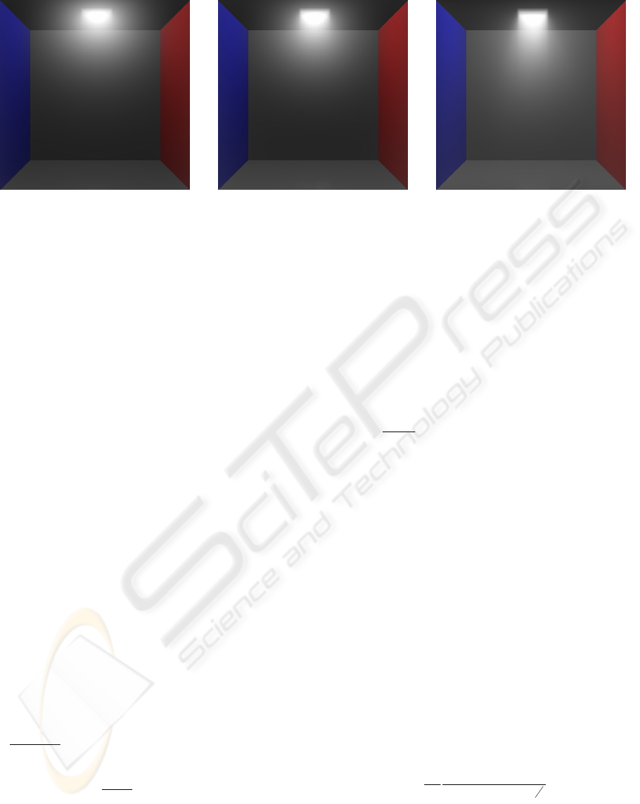
Figure 1: The appearance of participating media changes as the medium density is decreased from left to right. Multiple
scattering appears distinctive in the image on the left and is less obvious in the one on the right. Results are produced by
the proposed method at 2fps. The scene is illuminated by area light.
propose a method to solve the transport equation in
volume represented by grids rather than particles. As
a result, the calculation for the light scattering paths
is avoided. With this approach, we realize rendering
dynamic scenes.
Separable decomposition technique was
introduced by (Kautz, 1999), and it has been used
for BRDF rendering. Later (Wang, 2004) and (Liu,
2004) applied singular value decomposition (SVD)
to glossy BRDFs in PRT. In addition, (Wang, 2005)
introduced SVD to the approximation of BSSRDFs
by separating Henyey-Greenstein (HG) phase
function. Similarly, our proposed method
decomposes HG phase function in the rendering of
multiple scattering in participating media in order to
accelerate the computation.
2 BACKGROUND
2.1 Multiple Scattering in Participating
Media
When light travels in participating media, its
radiance undergoes changes due to emission, in-
scattering, absorption and out-scattering. The former
two phenomena increase the radiance, while the
latter two reduce it. The differential transport
equation of radiance
L in distance dx
r
is:
The increased radiance by emission can be
expressed as
() ()
e
L
x
x
α
κ
rr
, where
()
e
L
x
r
is the
emission density, and
()
x
α
κ
r
is the absorption
coefficient, which is related to the density of
participating media at point
x
r
.
·Absorption and out-scattering are respectively
represented by
()()
x
Lx
α
κ
r
r
and
()()
s
x
Lx
κ
rr
, where
()Lx
r
is the radiance at point
x
r
.
()
s
x
κ
r
is the
scattering coefficient, and it is also related to density.
· In-scattering is due to photons originally
moving in a certain direction being scattered into the
considered direction. The number of scattered
photons from differential solid angle
i
d
ω
σ
equals to
where
0
(,)
i
p
ω
ω
is the phase function. The phase
function can be interpreted as the scattered intensity
in direction
0
ω
, divided by the intensity that would
be scattered in that direction if the scattering were
isotropic (i.e. independent of the direction).
Ω
denotes the set of directions on the sphere around
point
x
r
.
The simplest phase function is the isotropic one.
Rayleigh phase functions are used to model
scattering processes produced by spherical particles
whose radii are smaller than around one-tenth the
light wavelength, while Mie phase functions are
generally used when particle size is comparable to
the radiation wavelength (Cerezo, 2005). In this
paper, we take scattering in clouds and fog as
examples, so the simple mathematical
approximation of Mie phase functions, HG phase
functions(Henyey, 1940)(Cornette, 1992), is used in
our transport light model. The HG phase function is:
where
(1,1)g
∈
−
is the media property describing
how strongly the media scatters forward or
backward, and
θ
denotes the angle between
i
ω
and
0
ω
.
0
00
00
(, )
() (, ) ()(, )
()
()(, ) (, )( , )
4
i
e
emission absorption
s
sii
out scattering
in scattering
dL x
xL x xLx
dx
x
xLx Lx p d
αα
ω
ω
κωκω
κ
κω ωωωσ
π
Ω
−
−
=−
−+
∫
r
rr rr
r
14424431442443
r
rr r
1442443
144444
2
444443
(1)
0
()
(, )( , )
4
i
s
ii
x
Lx p d
ω
κ
ω
ωω σ
π
Ω
∫
r
r
(2)
()
2
3
2
2
11
()
4
12cos
g
p
gg
θ
π
θ
−
=
+−
(3)
INTERACTIVE RENDERING OF MULTIPLE SCATTERING IN PARTICIPATING MEDIA USING SEPARABLE
PHASE FUNCTION
263
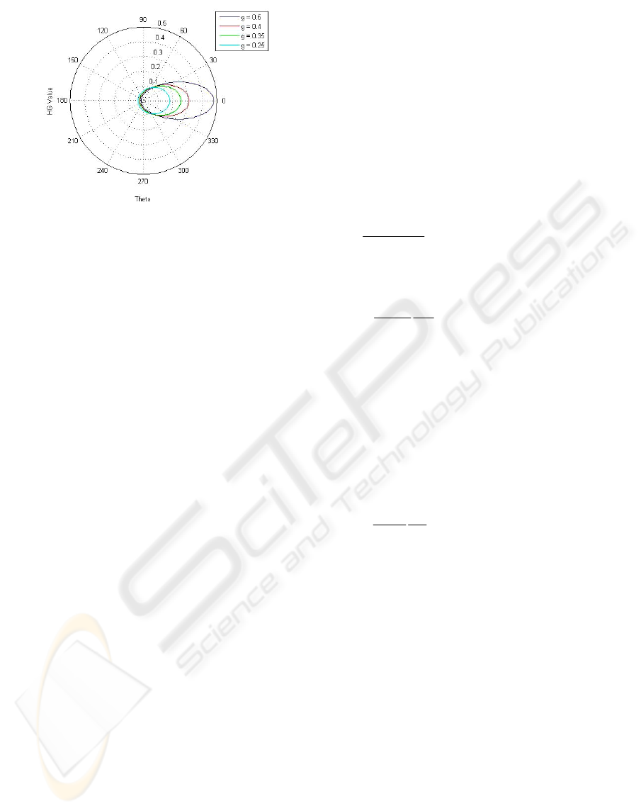
Figure 2: Phase Function (3).
The scattering properties of materials is depicted
with the Figure 2, which is a plot of HG Phase
function (3), where
g
is respectively 0.5, 0.4, 0.35,
and 0.25.
2.2 Singular Value Decomposition
(SVD) Factorization
In Mathematics, separable decompositions can
approximate (to arbitrary accuracy) a high-
dimensional function
f
with a sum of products of
lower-dimensional functions
k
g and
k
h :
Separable decompositions are usable for
remarkably compressing the original function
f
when a good approximation can be found with a
small
N
. In addition, they are capable of dividing
variables into separate expressions, namely
k
g
and
k
h
. Further calculation which involves one
variable may not need to refer to function
f
but to
only one of the post-decomposition functions
k
g or
k
h instead. Redundant calculation can be avoided
by adopting separable decompositions.
With the introduction of separable
decomposition into pre-computing phase function in
radiant Equation (1), the calculation speed is
expected to be drastically enhanced. In this paper,
we adopt the SVD method of decomposing phase
function in order to considerably reduce the
rendering time. We use SVD because it can produce
relatively optimal approximations (Kautz, 1999).
SVD of matrix
A
is the factorization that
T
A
USV=
,
where
[
]
k
Uu=
,
[
]
k
Vv=
and
(
)
k
Sdiag
ξ
=
. S is a
diagonal matrix of singular values
k
ξ
. As a result,
after SVD, each function
(, )
f
xy
can be
approximated as:
3 THE PROPOSED METHOD
In this section, we elaborate our method for
approximating transport equation using separable
phase functions. We also present error estimation of
our approximation compared with the original phase
functions.
3.1 Discretization of the Transport
Equation
The transport Equation (1) can be discretized into
the form
where
D is the number of sample directions. The
above equation can be solved by iterations. Suppose
at iteration step
n , we have the light radiance ()
n
Lx
r
,
the light radiance of step
1n
+
can be obtained after
one iteration:
where
() () ()
ts
x
xx
α
κ
κκ
=
+
r
rr
. For physically
visible materials, this iteration is convergent.
3.2 Separable Phase Function and
Error Estimation
3.2.1 Factorizing the Phase Function
In the general phase function
0
(,)
i
p
ω
ω
,
0
ω
represents the incident light, and
i
ω
is the arbitrary
outgoing light. We can sample the
D
directions in
the whole direction space and construct a
DD
×
matrix
A . Each element in column
0
ω
and row
i
ω
of
A
represents the value of
0
(,)
i
p
ω
ω
. We apply
SVD on
A and obtain:
SVD approximates the multivariate phase
function
0
(,)
i
p
ω
ω
as a sum of products of functions
1
(, ) () ()
N
kk
k
f
xy g xh y
=
≈
∑
(4)
1
(, ) () ()
N
kk k
k
f
xy u xv y
ξ
=
≈
∑
.
(5)
0
0
00
0
1
(, )
() (, )
()(, ) ()(, )
()
4
(, ) ( , )
4
e
emission
s
absorption out scattering
D
s
dd
d
in scattering
dL x
xL x
dx
xLx xLx
x
Lx p
D
α
α
ω
κω
κ
ωκ ω
κ
π
ω
ωω
π
−
=
−
≈
−−
+
∑
r
rr
r
1442443
rr rr
1
442 4 431442 4 43
r
r
1
444442444443
(6)
1
00
00
&
0
1
(,)(,)
() (, ) () (, )
()
4
(, ) ( , )
4
nn
n
et
emission out scattering absorption
D
n
s
dd
d
in scattering
Lxdx Lx
x
Lx dx xLx dx
x
Lx p dx
D
α
ωω
κωκω
κ
π
ωωω
π
+
−
=
−
+≈ +
−
+
∑
r
rr
r
rrrrr
1
444
2
4443144
2
443
r
r
r
1
444444
2
4444443
(7)
00
1
(,) ()().
N
ikkki
k
puv
ω
ω
ξ
ωω
=
≈
∑
(8)
GRAPP 2007 - International Conference on Computer Graphics Theory and Applications
264
k
u and
k
v
of lower dimensionality. In Equation (8),
N
is the number of terms used in approximation. By
this approach, phase function is divided into two
parts
0
()
k
u
ω
and
()
ki
v
ω
, which are only pertinent
with
i
ω
and
0
ω
respectively. Consequently, the
phase function is approximated by a few low-order
terms. Each of them can be represented by a 2D
texture map
0
()
kk
u
ξ
ω
or
()
kk i
v
ξ
ω
respectively
indexed by the incident direction
0
ω
or an outgoing
direction
i
ω
in
Ω
. We name
0
()
kk
u
ξ
ω
incident-
direction map and
()
kk i
v
ξ
ω
outgoing-direction
map.
We observe that
0
(,)
i
p
ω
ω
only varies with the
angle between
0
ω
and
i
ω
, so
A
should be real
symmetric. Symmetric matrix
A can be diagonalized
into the form
T
A
QMQ=
, where diagonal element of
M
are the eigenvalues of
A
, and the column
vectors of
Q are the corresponding eigenvectors. As
described in Section 2.2, matrix
A
can be factorized
with SVD into
T
A
USV=
. In this case,
UVQ
=
=
and
SM=
, so
0
()
kk
u
ξ
ω
and
()
kk i
v
ξ
ω
should
only differ by the sign.
After applying SVD to the phase function, the
iterative transport equation is transformed into,
3.2.2 Error Estimation of SVD
Approximation
SVD can be applied to general phase functions, and
the approximation can be arbitrarily accurate. We
are going to demonstrate the result of our
approximation of phase functions with cloud
rendering. In this case, HG phase functions
(Equation (3)), are most frequently adopted.
Therefore, we present the root mean squared error
(RMES) of SVD approximation for HG phase
functions here. We apply SVD to HG phase
functions and obtained the RMES, which is shown
in Figure 3.
From the bellow figure, the approximation takes
greater number of terms to achieve certain accuracy
as
g
grows. The RMSE of SVD is about 10% for
approximations of 24 terms when
g
equals 0.5. It is
a numerically acceptable approximation, and it is
used for cloud rendering in this paper.
Relative RMSE of HG SVD
0
0,1
0,2
0,3
0,4
0,5
0,6
0,7
0,8
1 3 5 7 9 111315171921232527
Number of Approximated Terms
RMSE
g = 0.25
g = 0.35
g = 0.40
g = 0.50
Figure 3: Relative RMSE of HG SVD.
4 IMPLEMENTATION
4.1 Precomputation
We use the software MATLAB for precalculating
the SVD results of phase functions. The incident-
direction map
0
()
kk
u
ξ
ω
and outgoing-direction
map
()
kk i
v
ξ
ω
are precomputed and respectively
stored in textures: Incident-Direction Texture and
Outgoing-Direction Texture. Both of them are 2D
textures indexed by column number
(1, )kN∈ and
row number
(1, )iD
∈
In Figure 4, we plotted the original HG phase
function values and the approximated HG phase
function values after applying SVD, using 8 and 24
approximating terms respectively.
4.2 Runtime Rendering Pipeline
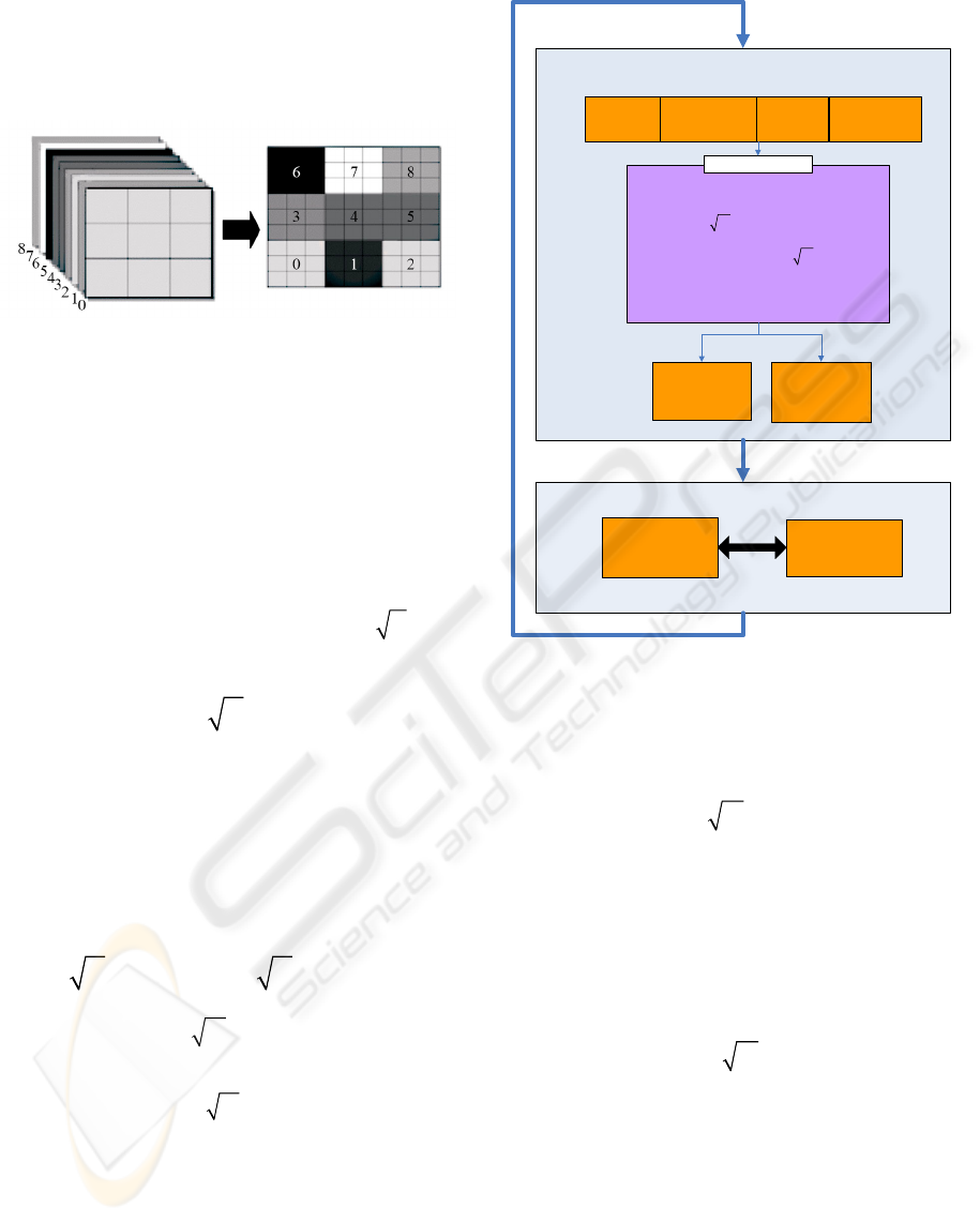
We represent our grids with what is called a flat 3D
texture (Harris, 2003). A flat 3D texture represents
actually a 3D volume, as shown in Figure 5. Flat 3D
textures can be updated in a single rendering pass.
Figure 4: Original HG Phase Function and SVD-
Approximated HG Values Plotted Using 8 and 24 Terms.
1
00
00
&
0
11
(,)(,)
() (, ) () (, )
()
4
() (, ) ()
4
nn
n
et
emission out scattering absorption
ND
n
s
kk d kk d
kd
in scattering
Lxdx Lx
xL x dx xL x dx
x
uLxvdx
D
α
ωω
κωκω
κ
π
ξω ωξω
π
+
−
==
−
+≈
+−
+
∑∑
rr r
rr r rr r
14442 4 4431442443
r
rr
144444444424444444443
(9)
INTERACTIVE RENDERING OF MULTIPLE SCATTERING IN PARTICIPATING MEDIA USING SEPARABLE
PHASE FUNCTION
265
This means that a 3D simulation can be
implemented in the same number of passes as that
required by an equivalent 2D simulation. Thus, it
provides a quick and inexpensive way to perform 3D
simulation.
(a) (b)
Figure 5: 3D texture (a) and its corresponding flat 3D
texture (b).
This section presents the rendering pipeline with
hardware acceleration during runtime. In every pass
of fragment program, we input Density Texture,
Radiance Texture, Incident Texture and Outgoing
Texture at iteration step
n
to update the values of
step
1n +
. The Density Texture and the Radiance
Texture respectively contain the density and
radiance values at each point in the rendering
volume. The Incident Texture indexes
0
()
kk
u
ξ
ω
with
k , and the Outgoing Texture contains the value
of
for each
k at each point. The rendering pipeline at
runtime is illustrated in Figure 6.
For each iteration, the process runs through the
fragment program a number of
D
times. During
each pass of fragment program, the radiance
1
0
(,)
n
Lxdx
ω
+
+
rr
in direction
(1, )dD∈
is updated
with Equation (9), and
0
11
() (, ) ()
ND
n
kk d kk d
kd
uLxvd
x
ξω ωξω
==
∑∑
r
r
(11)
is also calculated.
0
()
kk
u
ξ
ω
is indexed from
Incident Texture, and
is indexed from Outgoing Texture. In this way, the
original integral calculation:
in Equation (9) is avoided by simply retrieving
values from a texture.
Figure 6: Implementation Pipeline.
It remarkably reduces required calculation amount
during every rendering pass, thus the rendering
speed is considerably increased. At the same time,
1
(, ) ( )
n
dkkd
Lx v
ω
ξω
+
r
(14)
is added to the Temporary Outgoing Texture for
each
(1, )kN
∈
, and d is increased afterwards.
When
d reaches D , an iteration is complete. Thus
1
0
(, )
n
Lx
ω
+
r
in all D directions has been updated.
Meanwhile, the value of each grid in the Temporary
Outgoing Texture has been updated to be
Temporary Outgoing Texture and the Outgoing
Texture are switched for the next iteration. Iteration
continues, and eventually
1
0
(, )
n
Lx
ω
+
r
differs little
with
0
(, )
n
Lx
ω
r
, which indicates the convergence of
iteration.
1
(, ) ( )
D
n
dkkd
d
Lx v
ω
ξω
=
∑
r
(10)
1
(, ) ( )
D
n
dkkd
d
L
xvdx
ωξ ω
=
∑
rr
(12)
0
1
(, )( , )
D
dd
d
Lx p
ω
ωω
=
∑
r
(13)
1
1
(, ) ( )
D
n
dkkd
d
Lx v
ω
ξω
+
=
∑
r
(15)
Density
Texture
Outgoing
Texture
Temporary
Outgoing
Texture
Fragment Program
00
1
1
1
1
1. Update ( , ) with ( , ) and
(, ) ( )
2. Accumulate ( , ) ( )to
Temporary Outgoing Texture
3. Increase
k
k
nn
D
n
dkd
d
n
dkd
n
Lx Lx
Lx v
Lx v
d
ωω
ξ
ξ
ωω
ωω
+
=
+
+
∑
Incident
Texture
ACCUMULATE
Loop of (1, )dD
∈
Radiance
Texture
t
1
Radiance
Texture
n
+
UPDATE
Temporary
Outgoing
Texture
Outgoing
Texture
SWITCH
GRAPP 2007 - International Conference on Computer Graphics Theory and Applications
266
5 RESULTS AND DISCUSSIONS
The proposed technique has been implemented in
Direct3D/HLSL environment and run on an
NV7800GT graphics card. The volume resolution is
64 64 64××
.
In Figure 1, we demonstrate the appearance of
multiple scattering in participating media with
different uniform densities. The scene is illuminated
with parallel light rays travelling downwards from a
window in the ceiling. The number of discrete
directions,
D , is 128. The albedo is 0.9. The
multiple scattering is more representative in medium
with a larger density, while single scattering
dominates the scene of smaller density. We compute
one iteration in each frame, and when the uniform
density changes, we take the solution of the previous
frame as the initial value of the iteration, which
results in fast convergence. The scene is simulated
as 2fps. A dynamic scene is rendered interactively.
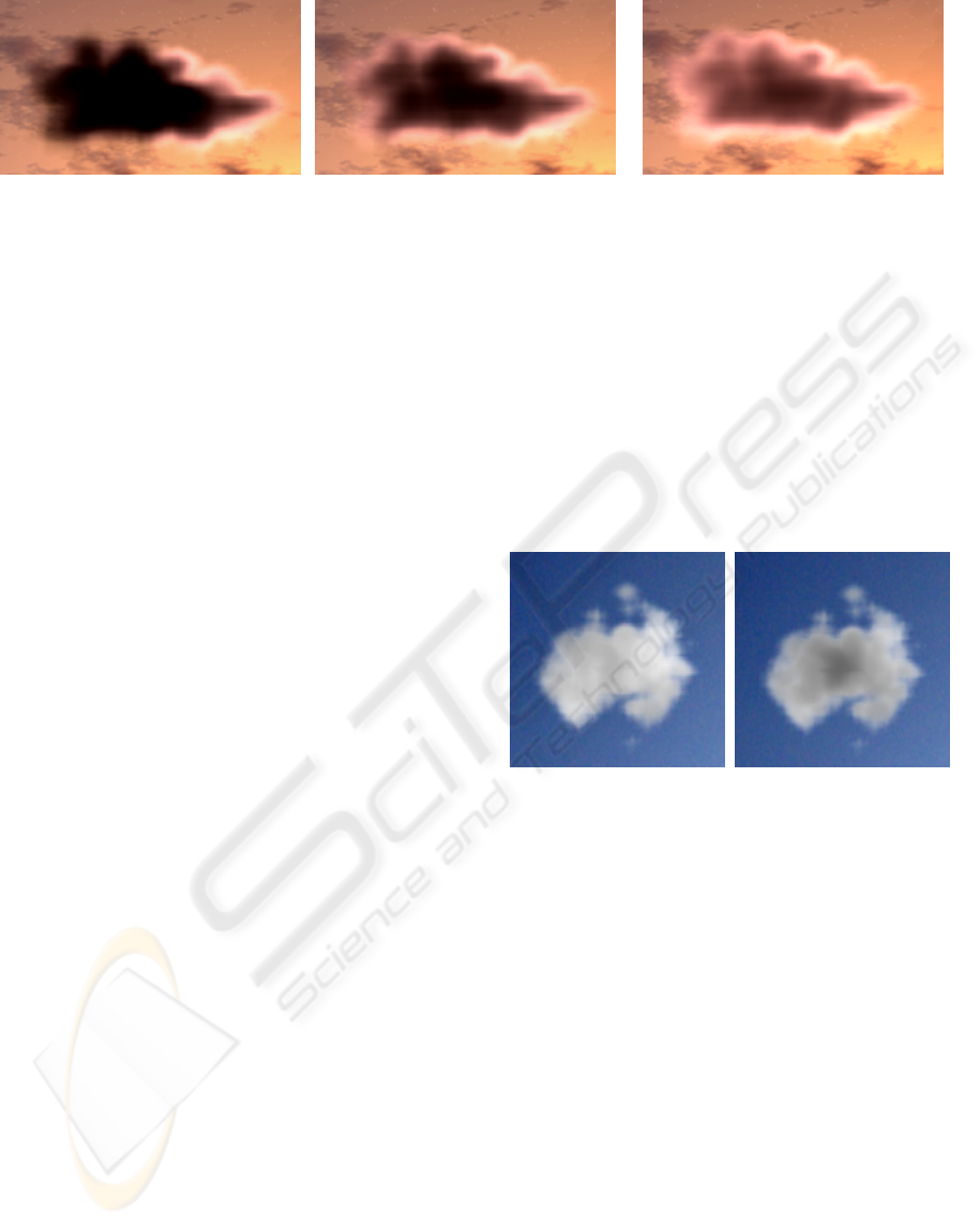
In Figure 7, we follow the converging process of
a piece of cloud after different iteration steps. The
image on the left displays the cloud after 20
iterations. At that time, the part closer to the sun is
firstly illuminated. In the images in the middle, the
energy gradually transports to other parts of the
cloud. Notice that the thicker part of the cloud
appears darker because of high extinction. The
image on the right shows the final stable appearance
of the cloud, which indicates the convergence of
transport equation. The number of discrete
directions
D is 256, and 1.5fps was achieved.
In Figure 8, we present an example of HG phase
function factorized by SVD. The image on the left is
rendered without factorizing the phase function. On
the right is an image shaded with our method, using
24-term SVD approximation.
g
is 0.5 in both
simulations. From the comparison, the cloud appears
a little darker in our proposed model, especially in
the thick part. It is due to that the reconstructed
value of the phase function with our method is
generally smaller than the original one, and phase
function is only related to the in-scattering part of
the transport equation. Therefore, the approximated
in-scattering energy is smaller than the actual value.
However, a rendering speed of 1.5fps is achieved
with the proposed algorithm compared with 0.2fps
of the unfactorized model. Moreover, visually good
results are obtained by the approximation. With our
approach, rendering speed is considerably enhanced,
while realism is mostly preserved.
Original N = 24
Figure 8: SVD factorization example, illuminated by the
sun.
6 CONCLUSIONS
We have presented a method for interactively
rendering multiple scattering in participating media
with little physics simplification and constraints on
media type. Compared with the Monte Carlo
rendering method, our approach achieves much
higher rendering speed. Meanwhile, compared with
other near real-time algorithms, such as (Harris,
2001) and (Sloan, 2002), ours has little constraints
on the lighting conditions. The material properties
and the scattering phase function. We approximate
phase functions in transport equation with singular
value decomposition. Using the proposed algorithm,
rendering of dynamic scenes can be implemented
with grid system. This technique greatly reduces the
required calculation amount and enhances the
20 iterations 40 iterations 60 iterations
Figure 7: A cloud illuminated at sun set. The images show appearances of the cloud with different iteration steps.
INTERACTIVE RENDERING OF MULTIPLE SCATTERING IN PARTICIPATING MEDIA USING SEPARABLE
PHASE FUNCTION
267

rendering speed. The proposed method successfully
models dynamic scenes that do not change rapidly.
However, as to highly dynamic scenes, the
transport equation takes more time to converge.
Once the change occurs before the convergence,
error appears and accumulates successively.
Therefore, we plan to focus on developing a
better model which converges faster in future work.
ACKNOWLEDGEMENTS
This research is supported by 973 program of China
under grant 2002CB312101, the National Natural
Science Foundation of China under grant 60603076
and 60475013.
REFERENCES
Cerezo, E., Pérez, F., Pueyo, X., Seron, F. J., Sillion, F. X.,
2005. A Survey on Participating Media Rendering
Techniques. In The Visual Computer 21, pp. 303-328,
2005.
Cornette W., Shanks J., 1992. Physical reasonable analytic
expression for single-scattering phase function.
Applied Optics 31, 16, 31–52, 1992.
Harris, M. J., Lastra, A., 2001. Real-Time Cloud
Rendering. In Proceedings of Eurographics 2001,
20(3):76-84, September 2001.
Harris, M. J., Baxter W. V. III, Scheuermann T., Lastra
A.. Simulation of Cloud Dynamics on Graphics
Hardware. In Proceedings of Graphics Hardware
2003.
Hegeman, K., Ashikhmin, M., Premoze, S., 2005. A
Lighting Model for General Participating Media. In
Proceedings of ACM SIGGRAPH Symposium on
Interactive 3D Graphics and Games, April 2005.
Henyey, G., Greenstein, J., 1940. Diffuse radiation in the
galaxy. Astrophysical Journal 88, 70–73, 1940.
Jensen, H. W., Christensen, P. H., 1998. Efficient
simulation of light transport in scenes with
participating media using photon maps. In
Proceedings of ACM SIGGRAPH 98, 311--320.
Kautz, J., McCool, M., 1999. Interactive Rendering with
Arbitrary BRDFs using separable approximation. In
10th Eurographics Workshop on Rendering, 1999, pp.
255-268, 379 (colour plate).
Liu, X., Sloan, P.-P., Shum, H.-Y., Snyder, J., 2004. All-
Frequency Precomputed Radiance Transfer for Glossy
Objects. In Eurographics Symposium on Rendering
2004, pp.337-344, 2004.
Pattanaik, S. N., Mudur, S. P., 1993. Computation of
Global Illumination in a Participating Medium by
Monte Carlo Simulation. In The Journal of
Visualization and Computer Animation, 4(3):133–152,
July - September 1993.
Premože, S., Ashikhmin, M., Tessendorf, J.,
Ramamoorthi, R., Nayar, S., 2004. Practical rendering
of multiple scattering effects in participating media. In
Proceedings of the Eurographics Symposium on
Rendering 2004.
SLOAN, P.-P., KAUTZ, J., SNYDER, J., 2002.
Precomputed radiance transfer for real-time rendering
in dynamic, low-frequency lighting environments. In
ACM Transactions on Graphics 21, 3 (July), 527–536.
Szirmay-Kalos, L., Sbert, M., Ummenhoffer, T., 2005.
Real-Time Multiple Scattering in Participating Media
with Illumination Networks. In Proceedings of the
Eurographics Symposium on Rendering 2005.
Wang, R., Tran, J., Luebke, D., 2004. All-frequency
relighting of non-diffuse objects using separable
BRDF approximation. In Proceedings of
Eurographics Symposium on Rendering 2004, pp.345–
354, 2004.
Wang, R., Tran, J., Luebke, D., 2005. All-frequency
interactive relighting of translucent objects with single
and multiple scattering. In ACM Transactions on
Graphics, 24(3): 1202-1207.
GRAPP 2007 - International Conference on Computer Graphics Theory and Applications
268
