
Frame-Frame Matching for Realtime Consistent Visual
Mapping
Kurt Konolige
1
and Motilal Agrawal
1
1
Artificial Intelligence Center, SRI International, 333 Ravenswood Ave.
94025 Menlo Park, USA
Abstract. Many successful indoor mapping techniques employ frame-to-frame
matching of laser scans to produce detailed local maps, as well as closing large
loops. In this paper, we propose a framework for applying the same techniques
to visual imagery, matching visual frames with large numbers of point features.
The relationship between frames is kept as a nonlinear measurement, and can
be used to solve large loop closures quickly. Both monocular (bearing-only)
and binocular vision can be used to generate matches. Other advantages of our
system are that no special landmark initialization is required, and large loops
can be solved very quickly.
1 Introduction
Visual motion registration is a key technology for many applications, since the sen-
sors are inexpensive and provide high information bandwidth. In particular, we are
interested in using it to construct maps and maintain precise position estimates for a
mobile robot platform indoors and outdoors, in extended environments over loops of
> 100m, and in the absence of global signals such as GPS – this is a classic SLAM
(simultaneous localization and mapping) problem.
In a typical application, we gather images at frame rates, and extract hundreds of
features in each frame for estimating frame to frame motion. Over the course of 100
m, moving at 1 m/sec, we can have a thousand images and half a million features.
The best estimate of the frame poses and feature positions is then a large nonlinear
optimization problem. In previous research using laser rangefinders, one approach to
this problem was to perform frame-to-frame matching of the laser scans, and keep
only the constraints among the frames, rather than attempting to directly estimate the
position of each scan reading (feature). This technique is used in the most successful
methods for large-scale LRF map-making, FastSLAM 1117 and Consistent Pose
Estimation 8121516. Using matching instead of feature estimation reduces the size of
the nonlinear system by a large factor, since the features no longer enter into it.
In this paper, we present a frame-to-frame method for constructing maps from vis-
ual data. The main purpose of the paper is
• To show that precise realtime estimation of pose is possible, even in difficult
Konolige K. and Agrawal M. (2007).
Frame-Frame Matching for Realtime Consistent Visual Mapping.
In Robot Vision, pages 13-26
DOI: 10.5220/0002068800130026
Copyright
c
SciTePress
outdoor environments, by visually matching frames that are spatially close (and
not just temporally close, as in visual odometry).
• To show that a nonlinear frame-frame system is capable of quickly solving
large-scale loop closure from visual information.
Precise estimation of frame pose is important in constructing good maps. In visual
odometry, the pose is estimated by matching image features across several consecu-
tive frames 11819. Current techniques achieve very precise results, but pose errors
grow unbounded with time, even when the camera stays in the same area, because
there is no matching of frames that are close in space, but not time. In contrast, the
frame-frame matching techniques for LRF maps look for matches between frames
that are spatially close, and obtain very precise floorplan results (see
Fig. 1). In a
similar manner, our system computes the structure of spatially-coherent frame-frame
visual constraints, and optimizes incrementally for realtime performance.
Recent research in vision-based SLAM has concentrated on solving the pose esti-
mation problem for small areas by keeping track of feature positions. Davison’s
innovative technique 2 used a combined EKF over a small set of features. More
recently, several approaches use a large number of features, each with its own inde-
pendent EKF 4232122. These methods rely on novel techniques for matching against
a large database of features to achieve realtime performance. In both cases, the pose
estimation accuracy suffers because of mismatches and imprecision in feature local-
ization. We are investigating the relative performance of these techniques in small
areas against our frame-frame matching, but do not yet have results to report here.
One advantage of the frame system is that no special initialization is required for
landmarks, even in the monocular case, since we do not track the 3D position of
landmarks. Instead, we use standard techniques in structure from motion to match
image features and solve a projective system for the optimum local registration of
frames and features 191025. Our novel technique is to derive a synthetic nonlinear
measurement among frames alone that summarizes the registration. One obstacle to
frame-frame constraints in the monocular case is that they are only partially con-
strained (up to scale) – current laser scan systems, for example, cannot handle this
case 13. Our technique is more general, and can handle projective or even less-
constrained cases.
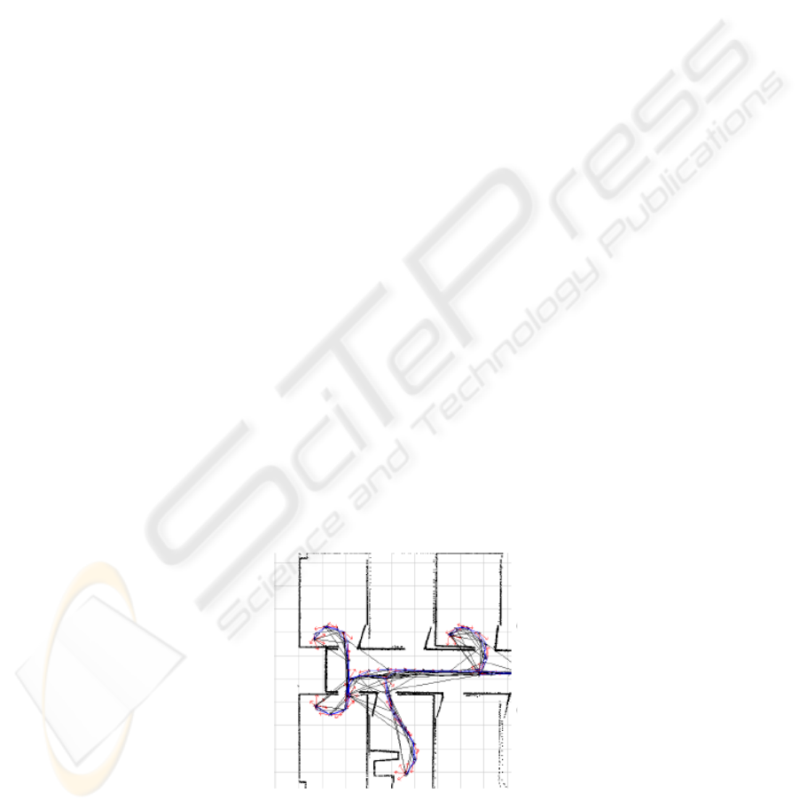
Fig. 1. Frames linked by matching laser scans. Red arrows are frames, lines are links. When-
ever there is a significant overlap of scans, a link is inserted, e.g., when the LRF sees through
a doorway into the hall from separate rooms.
14

The frame-frame constraints are linked into a nonlinear system that mimics the
much larger frame+landmark system. One of the weaknesses of current visual SLAM
techniques with large numbers of landmarks is closing larger loops. In the course of
a 100 m loop, there can be significant drift even with good frame-frame matching – in
typical outdoor terrain our system has 2-4% error. After finding a loop-closing
match, the frames in the loop can experience significant dislocation from their initial
values. Our system computes the optimal nonlinear solution to the frame poses, in a
fraction of a second, for large frame sets (> 1K frames).
Similar work in large-scale loop closure has recently emerged in undersea mapping
using cameras 2024 26, although not in a realtime context. This research also uses
frame-frame matching of images that are spatially close, but then filters the frame
constraint system using a sparse information filter. In contrast, we construct an ap-
proximate nonlinear system, which can better conform to loop-closing constraints.
2 Visual Matching and Nonlinear Systems
Our approach derives from structure from motion theory of computer vision, in par-
ticular Sparse Bundle Adjustment (SBA). Of necessity we will present a short over-
view to introduce notation, and then apply it to frame-frame matching and the con-
struction of the frame constraint system. Readers are urged to consult the excellent
review in 25 for more detailed information.
2.1 Sparse Bundle Adjustment
We wish to estimate the optimal values of a set of parameters x, given a set of meas-
urements
z
. A measurement function )(xz describes the expected measurement
from a given configuration of parameters x. The error or cost induced by a given
parameter set is
)(xzz −=
ε
. (1)
If there are a set of independent measurements z
i
, each a Gaussian with covariance
1−
i
W , then the MLE estimate x
ˆ
minimizes the cost sum
∑
=
i
ii
T
i
WE
εε
. (2)
Since (2) is nonlinear, solving it involves reduction to a linear problem in the vicinity
of an initial solution. At a value x, f can be approximated as
xxxxxx
δδδδ
Hgff
TT
2
1
)()( ++≈+ , (3)
where g is the gradient and H is the Hessian of f with respect to x. The minimum of f
is found by equating the derivative to zero. A further approximation gets rid of the
second-derivative Hessian terms in favor of the Jacobian
xz
∂
∂
≡
J (the Gauss-
Newton normal equations):
0
εδ
WJWJJ
TT
−=x , (4)
with W the block-diagonal matrix formed from all the individual W
i
. In the nonlinear
15

case, one starts with an estimate x
0
, and iterates the linear solution until convergence
to an estimate
x
ˆ
. The Hessian has been approximated by
WJJH
T
≈ . (5)
It should be noted that
H
ˆ
is also the inverse of the covariance of x
ˆ
, that is, the in-
formation matrix.
The general linear system (4) can be solved using a variety of methods, paying at-
tention to step size to insure that there is a reduction in the total cost. In the applica-
tion of (4) to camera frames and point features, SBA takes advantage of the sparse
structure of H to derive an efficient decomposition. Consider a set of camera frames
p and features q. The measurement functions
),(
jiij
qpz
are the projection of fea-
tures q
j
onto the frames p
i
. Since only a small, bounded number of all features are
seen by any camera frame, the pattern of the Jacobian
xz
∂
∂
is very sparse (the pri-
mary structure). If we reconstruct (4) by ordering the frames first and the features
second, we get the following block structure:
⎥
⎥
⎦
⎤
⎢
⎢
⎣
⎡
−
−
=
⎥
⎦
⎤
⎢
⎣
⎡
⎥
⎦
⎤
⎢
⎣
⎡
qq
T
q
pp
T
p
qqqp
pqpp
WJ
WJ
HH
HH
ε
ε
δ
δ
q
p
, (6)
where H
pp
and H
qq
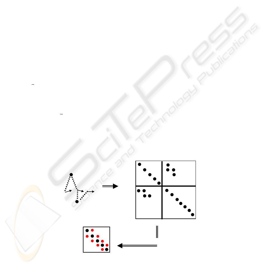
are block-diagonal. Figure 2 shows a small example of three
frames and two features.
Since the number of features is normally much larger than the number of frames,
(6) would be easier to solve if it consisted just of the H
pp
section. In fact, it is possi-
ble to reduce (6) to the form
gH
pp
−=p
δ
, (7)
where
qq
T
qqqpqpp
T
p
qpqqpqpppp
WJHHWJg
HHHHH
εε
1
1
−
−
−≡
−≡
(8)
After solving the reduced system (7) for the p’s, the results can be back-propagated to
find the q’s, and the process iterated. Note that
pp
H is the inverse covariance of the
frame pose estimate.
It is important that in our application, the Hessian of the reduced system remains
sparse as the number of frames grows (
Fig. 2, bottom). This is because each feature is
seen by only a small, bounded number of frames, and so the number of elements of
pp
H grows only linearly with the number of frames.
Another characteristic of the system (7) is that the choice of origin is arbitrary.
All of the measurements are relative to a frame, and are preserved under arbitrary
rigid transformations. So we can take any solution of (7) and transform it to a par-
ticular coordinate system, or equivalently, fix the pose of one of the frames. In fixing
the pose, we eliminate the frame parameters, but keep it in the measurement equation
as a fixed value for projection errors.
16
2.2 Frame-Frame Matching
So far, the development has been a standard exposition of SBA. We will use (8) to
calculate an incremental bundle adjustment 5 when adding a new camera frame to the
system. For a large system, however, full SBA becomes computationally expensive,
and more importantly, unstable when closing loops with significant offset. By using
the idea of frame-frame matching from the LRF SLAM literature, we can convert a
large nonlinear system of frame and feature measurements into a simpler (still nonlin-
ear) system of frame-frame constraints. This conversion is only approximate, but we
will show in a series of experiments that it produces good results.
Consider a simple system consisting of two frames p
0
and p
1
, along with a large set
of features q that are visible in both frames. Fix p
0
to be the origin, and calculate the
estimated value
1
ˆ
p and its inverse covariance
11
H
(from (8)) using SBA. These
two values summarize the complicated nonlinear relationship between p
0
and p
1
(con-
structed from the feature measurements) as a Gaussian PDF. This is exactly the PDF
we would get from the measurement and its associated function
1
11
ˆ
)(
pz
ppz
=
=
, (9)
with inverse covariance
11
H
(see Appendix I). Here the measurement itself is
1
ˆ
p ,
the estimated position of
1
p . So we have compressed the effect of all variables q and
their projections
z into a simple synthetic linear measurement on
1
p .
Unfortunately (9) only holds when
0
p is the origin. What we would like is a
measurement function that characterizes the relationship of
0
p and
1
p no matter
where
0
p is located. The easiest way to do this is to measure the position of
1
p in
Fig. 2. Top left: Three frames (arrows) and three features (dots). The dotted lines indicate that
a feature is viewed from a frame. The Hessian is on the right, with the nonzero elements
marked. Bottom left: reduced Hessian Hpp, showing banded structure.
p1 p2 p3
q
1
q
2 …
p1
p2
p3
…
q1
q2
…
p1
p2
p3
p1 p2 p3
p1
p2
p3
…
17

the frame
0
p . Changing from the global frame to
0
p ’s frame is accomplished by a
homogenous transformation (see 3); the value of
1
p in
0
p ’s frame is denoted
1
0
p .
Now the measurement and its function are
1
0
1
0
10
ˆ
),(
pz
pppz
=
=
, (10)
again with inverse covariance
11
H
. This measurement function is no longer linear in
the frame variables, but it is easy to see that when
0
p is the origin, it reduces to (9).
More importantly, (10) produces exactly the same PDF for
1
p as does SBA, when
both use the same (arbitrary) fixed value for
0
p (see Appendix I for a proof).
It is worth emphasizing the import of going from the large set of projective meas-
urements
),(
jiij
qpz to the single measurement
1
0
10
),( pppz = .
•
The nonlinear system is reduced from several hundred variables (the features plus
frames) to two variables (the frames).
•
The nonlinear nature of the system is preserved, so that it is invariant to the abso-
lute orientation and position of
0
p and
1
p . This is in contrast to working with a
reduced linear system (as in 20), where re-linearization to correct bad initial angles
is not possible.
•
The measurement function (10) is a good approximation of the original system, as
long as
1
0
p is close to
1
0
ˆ
p .
•
The measurement function (10) can be over-parameterized – the obvious case is
for a monocular camera, in which the relation between
0
p and
1
p can be deter-
mined only up to a scale factor. The inverse covariance
11
H
has a null space and
is not invertible, but is still useable in finding an ML estimate. This property is a
great benefit, since we don’t have to worry about finding a minimal representation,
and can use frame-frame measurements even when they are only partially con-
strained, e.g, in the monocular case.
There is nothing that restricts frame-frame matching to working with just two frames
– the reduction to pose differences works with any number of frames that have fea-
tures in common. One frame must be chosen as the origin (say
0
p ); the general form
is
⎥
⎥
⎥
⎥
⎥
⎦
⎤
⎢
⎢
⎢
⎢
⎢
⎣
⎡
=
⎥
⎥
⎥
⎥
⎥
⎦
⎤
⎢
⎢
⎢
⎢
⎢
⎣
⎡
=
nn
p
p
p
p
p
p
z
ˆ
ˆ
ˆ
,)(
0
2
0
1
0
0
2
0
1
0
##
zp
(11)
with inverse covariance
pp
H
. If all frames have at least one feature in common,
then
pp
H
has no nonzero elements, and the frames are fully connected.
18

3 Implementation
The goal of this research is to implement a system that builds a map in realtime from
visual information. The map system has the following elements:
1.
Map state is the estimated pose p
ˆ
of a set of frames that are extracted during
camera motion.
2.
Frame measurements are a set of measurements of the form (10) or (11).
3.
Image features are point features extracted at each frame, associated with the
frame. Image features do not enter into the map structure, and are kept only to per-
form image-to-image matching.
When a new frame is acquired, the system augments the map state
p
ˆ
, and computes
new frame measurements based on visual matching with other frames that are near in
time and space. Then, a portion of the system is optimized using a subset of the
frames and measurements. Where only local matches are made, a local area is opti-
mized; for larger loops, the whole system may be involved. The optimization then
updates the estimated pose
p
ˆ
.
3.1 Visual Matching
The system expects calibrated cameras, and can use either monocular or binocular
matching. For the binocular case, we match two frames; for monocular, three frames
are used to preserve the relative scale. In either case, we use simple Harris points,
and find putative matches by normalized cross-correlation of a small patch around the
point. A robust RANSAC method 6 is used to find a good motion hypothesis. In the
binocular case 181, three matched points are triangulated and then an absolute orien-
tation step is used to estimate the
3D motion. The estimate is scored by projecting all
features back onto the images and counting the number of inliers.
For monocular motion, the 5-point method of 18 is used to hypothesize an essential
matrix for the first and third frames, and the second frame is estimated from a three-
point resection 9. Again projection is used to find the maximum number of inliers.
For the best hypothesis, the SBA method of Section 2.1 optimizes the whole sys-
tem, and at the same time computes the Hessian for the frame-frame constraint (10) or
(11). Note that in the monocular case, the Hessian has a null space of dimension one,
since the overall scale is indeterminate. This exactly characterizes the relative place-
ment of the three frames, while leaving open the scale.
3.2 Data Association
Visual matching takes place independent of the state of the map system, producing
frame-frame measurements. One of the critical system choices is deciding which
measurements to add when a new frame is added. For this paper we adopted a simple
scheme that is efficient and produces reasonable results. First, we add a set of meas-
urements that connect to the previous
N frames, where N is a small number, typically
19

1 to 5. Then, we add at most one measurement to any close, non-recent frame. These
additions keep the map estimate consistent locally. Finally, we search for longer-
range measurements that close larger loops, and add one of these if appropriate.
For short-range motion, spatially nearby frames can be identified if they are close
in the graph of measurements 8. For longer-range loops, we are investigating the use
of more invariant features to reliably identify closure hypotheses, e.g., the method of
24.
3.3 Computation
The more demanding case is binocular, because features must be extracted from two
images, and matched across the images as well as with previous images.
Fig. pre-
sents a breakdown of the computation on a 2 GHz Core Duo Pentium M, using
512x384 images and approximately 500 points in each image. For each new frame,
the first three computations must be performed to connect to the previous frame. For
more matches to previous frames, only the motion estimation step needs to be done;
for matches to close frames, both feature tracking and motion estimation are needed.
The system can perform several visual matches within a 15 Hz cycle, with visual
matching partitioned between the two cores. Updating the map system takes very
little time compared to the matching stage:
Fig. also shows some timings for medium
to large systems. The system is implemented and runs on an outdoor robot that uses
stereo to autonomously build maps in off-road environments 14.
4 Results
We performed two sets of experiments, one with simulated data where the ground
truth is known, and one with a dataset from an outdoor robot moving about 100 m in
a loop.
Algorithm CPU time
Feature extraction and stereo matching 25 ms
Visual matching 24 ms
Motion estimation (per constraint) 16 ms
System optimization
80 frames 30 ms
330 frames 100 ms
660 frames 220 ms
1330 frames 340 ms
Fig. 3. Computation times for the main parts of the mapping system. 2 GHz Pentium M,
512x384 images, ~500 points per image.
20
4.1 Simulated Monocular System
In this experiment we compare the frame-frame system to the standard SBA method
on a local loop, to test its accuracy. The motion is circular, with the camera looking
in the direction of motion. For the frame system, we use 3-frame constraints to
propagate relative scale. We varied the density of constraints for each frame, from 1
to 5.
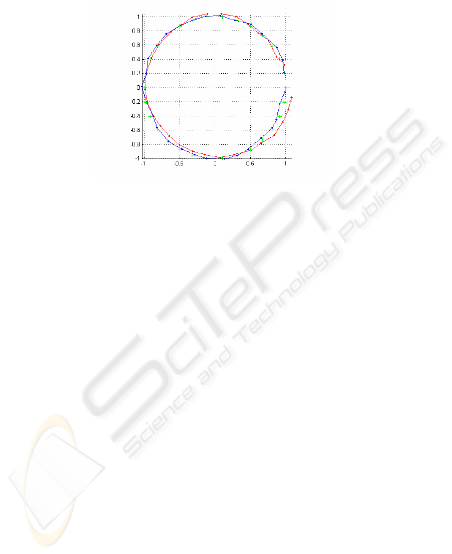
Fig. shows typical results, with the SBA motion in blue, and the frame system in
red. For the frame system, the last few frames were matched against the first few to
create loop constraints. For SBA, image feature tracks average 7 frames, and no
loop-closure matching is used. Note the accuracy of the frame system, even though it
uses several orders of magnitude fewer measurements.
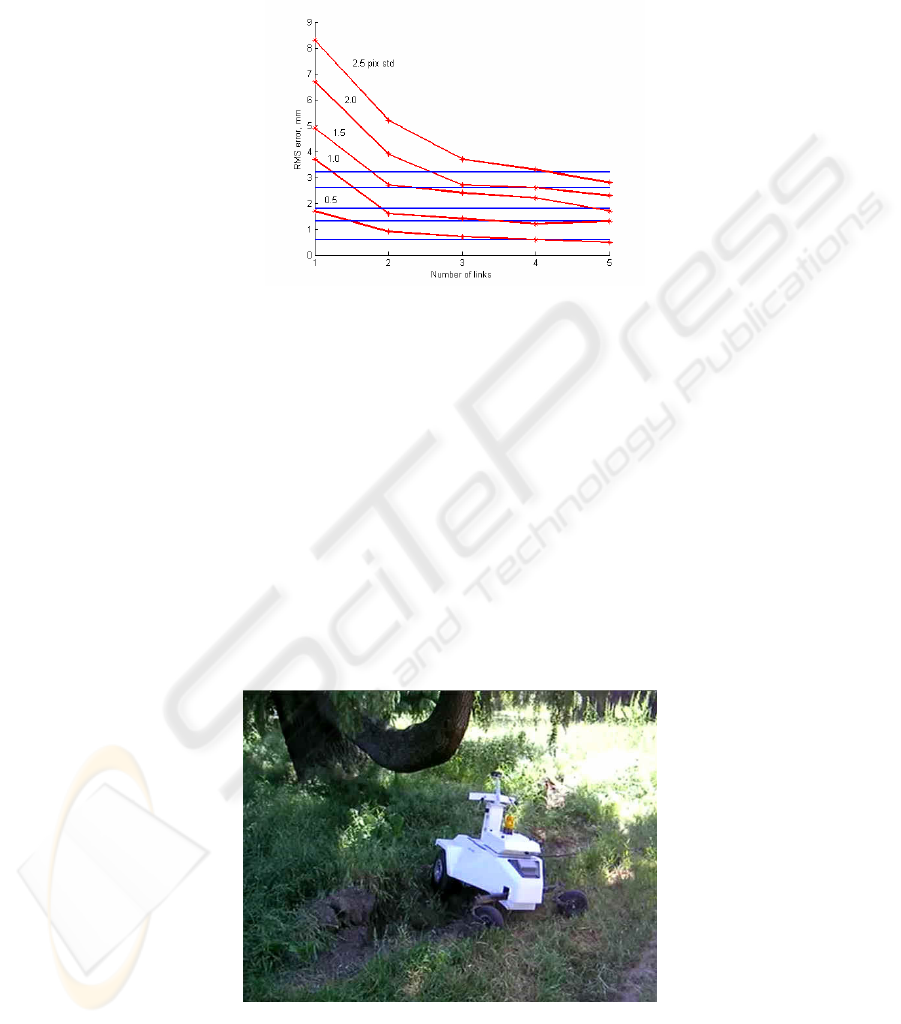
Figure 5 shows statistics for varying amounts of Gaussian noise on the image
points. The error is measured as the rms distance of poses from their ground-truth
positions, averaged over 20 runs. Since the scale and placement of the result is not
constrained, we did a final minimization step, using a rigid transformation and scale
to bring it into correspondence with ground truth.
The key aspect of Figure 5 is that the reduced system results are as good as or bet-
ter than SBA, especially at 4 and 5 links. As the image noise increases, SBA does
increasingly worse because it is open-ended, while the frame system degrades less.
Note that these results are much more accurate than the reduced system in 7, which
uses an averaging technique between adjacent frames, and neglects longer links. This
experiment validates the use of the frame system for high-accuracy motion estimation
in a local area.
Fig. 4. Typical circular motion estimate at high noise levels, projected onto the XY plane.
Green crosses are the ground truth frame positions. Blue is full SBA, red is the frame system
with 2 links (3 pixels image error).
21
4.2 Outdoor Stereo System
We conducted a large outdoor experiment, using a mobile robot with a fixed stereo
pair, inertial system, and GPS (
Fig. ). The FOV of each camera was about 100
0
, and
the baseline was 12 cm; the height above ground was about 0.5 m, and the cameras
pointed forward at a slight angle. This arrangement presents a challenging situation:
wide FOV and short baseline make distance errors large, and a small offset from the
ground plane makes it difficult to track points over longer distances.
The test course covered about 110 m, and concluded at the spot where it started.
Fig. 8 shows the global position, as determined by GPS and inertial systems, and the
poses computed from the frame system – 1172 frames with average spacing of just
Fig. 5. RMS error in pose (mm) for circular motion, for different numbers of links and image
noise. Red lines are frame system, blue lines are full SBA. Bottommost red and blue lines are
for 0.5 pixels image noise, topmost are for 2.5 pixels noise.
Fig. 6. Outdoor robot in typical terrain. Robot is part of a DARPA project, Learning Ap-
plied to Ground Robotics. Two stereo systems are on the upper crossbar.
22
under 0.1 m. The run started from the origin, went across and diagonally down to the
lower right, then came back below the original track. The frame system did a reason-
able job, with an accumulated error of about 3 m over the run. The angle gets off a
bit on the return trip, and consequently the loop meeting point is overrun. Note that
the travel distance was very close – 110.9 m for GPS, 110.02 for VO.
To correct the accumulated error, we closed the loop by matching the last frame to
the first. Our visual matching algorithm was used to find the constraint, since the two
frames were close. The visual results now track GPS much more closely (
Fig. ), and
in fact are better than GPS right around the origin, where GPS is off by almost 1 m.
The path length has not changed, but the angular error along the path has been cor-
rected and spread evenly, based on the loop closure.
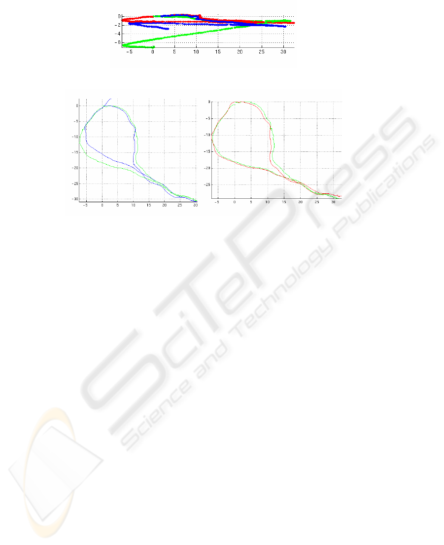
Even more interesting is the data from the Z (earth-normal) direction, in
Fig. . The
GPS/inertial data drifts considerably over the run, ending at almost -7m. The frame
data (blue) also drifts, but to much less extent, ending at -3 m. Adding loop closure
corrects the drift at the origin, and pulls up the rest of the path as well.
Given our timing results, it is possible to perform loop closure online. But we can
reduce the computational load still further by reducing the number of frame-frame
constraints. To do this, we use the same technique as in (6)-(8), but add to the fea-
tures
q all the frames between two endframes. The reduced system (7) then contains
just the two endframes, and we construct a synthetic measurement between these
two, as in (9). For this experiment, two reductions were chosen, based on 1m and 4m
distance. Starting with the first frame, we find the next frame that is greater than this
distance or more than 10
o
different in angle. We then reduce all frames in between,
add the loop closure constraint, and solve the system. The reduction leads to systems
of 126 and 41 poses, respectively. The results are shown in
Fig. . The blue crosses,
for the 126-frame system, recover almost exactly the form of the original frame sys-
Fig. 7. Comparison of Z vs. X motion of GPS (green), frame system (blue), and frame system
with loop closure (red).
Fig. 8. Top: Frame system of an extended outdoor run. Global pose from GPS and inertial
sensors (green), frame system in blue. Note the overshoot at the end of the loop. Bottom:
Frame system with loop closure, in red.
23
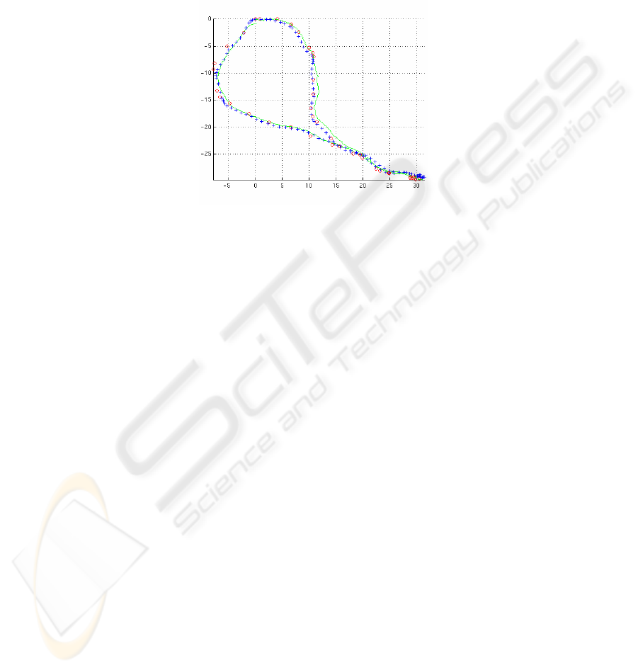
tem. Even with a 10-fold reduction in the number of frames, from 1172 to 126, the
system produces excellent results. With only 41 poses, errors start to appear at a
small scale, although the overall shape still remains very good.
5 Discussion
This paper lays the foundation for an online method of consistent motion estimation,
one that takes into account global constraints such as loop closure, while preserving
the fine structure of motion. It is based on proven methods from the laser scan-
matching SLAM literature, adapted using structure-from-motion techniques. A care-
ful analysis of the structure of measurements in SBA shows how to construct new,
nonlinear frame-frame constraints in a theoretically motivated way. The resultant
systems can be almost as accurate as the original system, while enjoying large speed-
ups in computation.
One of the nice properties of the frame-frame system is that it keeps the set of cam-
era frames, so that reconstruction (e.g., dense stereo) can be performed. This is in
contrast to EKF methods 14232122, which keep only a current estimate of the camera
pose.
While we show that online consistent estimation is possible, we have not yet de-
veloped a full system that exploits it. Such a system would have a map management
component, for keeping track of images associated with poses, and deciding when to
match the current image against others for loop closure. It would also need more
robust features for wide-baseline matching. It is our goal to construct a complete
system that performs online map-making over large areas, using just visual input.
Our current system uses the robust VO component to keep track of position in var-
ied outdoor terrain, including under tree cover where GPS does not work very well.
Our system performed the best in a final evaluation of the DARPA Learning Applied
to Ground Robotics project in June of 2006, using VO to keep track of its position
over a challenging course.
Fig. 9. Loop-closing with reduced number of poses. The blue crosses are for 1m distance
between frames (126 poses), the red circles for 4m (41 poses). Green is global GPS pose.
24

References
1. Agrawal, M. and Konolige, K. Real-time Localization in Outdoor Environments using
Stereo Vision and Inexpensive GPS. Proceedings of the International Conference on Pat-
tern Recognition (2006)
2. Davison, A. Realtime SLAM with a single camera. Proc. ICCV, 2003.
3. Craig, J.J. Introduction to robotics: mechanics and control, AddisonWesley, MA, 1989.
4. Eade, E. and T. Drummond, "Scalable Monocular SLAM," CVPR (2006).
5. Engels, C., H. Stewénius, D. Nistér. Bundle Adjustment Rules. Photogrammetric Computer
Vision (PCV), September 2006.
6. Fischler, M. and R. Bolles. Random sample consensus: a paradigm for model fitting with
application to image analysis and automated cartography. Commun. ACM., 24:381–395,
1981.
7. Govindu, V. M. Lie-algebraic averaging for globally consistent motion estimation. In
Proc. IEEE Conference on Computer Vision and Pattern Recognition, June 2004.
8. Gutmann, J. S. and K. Konolige. Incremental Mapping of Large Cyclic Environments. In
CIRA 99, Monterey, California, 1999.
9. Haralick, R., C. Lee, K. Ottenberg, M. Nolle. Review and analysis of solutions of the three
point perspective pose estimation problem. IJCV (1994).
10. Hartley, R. and A. Zisserman. Multiple View Geometry in Computer Vision, Second Edi-
tion. Cambridge University Press, 2003.
11. Hahnel, D., W. Burgard, D. Fox, and S. Thrun. An efficient FastSLAM algorithm for gen-
erating maps of large-scale cyclic environments from raw laser range measurements. In
Proc. of the IEEE/RSJ Int. Conf. on Intelligent Robots and Systems (IROS), 2003.
12. Konolige, K. Large-Scale Map Making. In Proc. AAAI, San Jose, California (2004).
13. Konolige, K. SLAM via variable reduction from constraint maps. In Proc. ICRA, March
2005.
14. Konolige, K., Agrawal, M., Bolles, R., Cowan, C., Fischler, M. and Gerkey, B. Outdoor
Mapping and Navigation using Stereo Vision. Proceedings of the International Symposium
on Experimental Robotics, Brazil (2006)
15. Lu, F. and E. E. Milios. Globally consistent range scan alignment for environment map-
ping. Autonomous Robots, 4(4), 1997.
16. Montemerlo, M. and S. Thrun. Large-scale robotic 3-d mapping of urban structures. In
ISER
, Singapore, 2004.
17. Montemerlo, M., Thrun, S., Koller, D. and Wegbreit, B. FastSLAM: A fac-
tored solution to the simultaneous localization and mapping problem. AAAI (2002).
18. Nister, D., O. Naroditsky, and J. Bergen. Visual odometry. In Proc CVPR, June 2004.
19. Olson, C. F., L. H. Matthies, M. Schoppers, and M. W. Maimone. Robust stereo ego-
motion for long distance navigation. In Proc CVPR, 2000.
20. Ryan, E., Singh, H., and J. Leonard, “Exactly sparse delayed state filters,” in Proc ICRA,
April 2005.
21. Se, S., Lowe, D. G., and J. J. Little. Vision-Based Global Localization and Mapping for
Mobile Robots. IEEE Transactions on Robotics, 21(3), June 2005.
22. Se, S., Lowe, D. G., and J. J. Little. Mobile robot localization and mapping with uncer-
tainty using scale-invariant visual landmarks, Int. J. Robot. Res.21(8), Aug. 2002.
23. Sim, R., P. Elinas, M. Griffin, and J. J. Little. Vision-based slam using the rao-
blackwellised particle filter. In IJCAI Workshop on Reasoningwith Uncertainty in Robotics,
2005.
24. Singh, H., C. Roman, O. Pizarro, and R. Eustice, Advances in high-resolution imaging from
underwater vehicles, Intl. Symp. on Robotics Research, October 2005
25

25. Triggs, B., P. McLauchlan, R. Hartley, and A. Fitzgibbon. Bundle adjustment - a modern
synthesis. In Vision Algorithms: Theory & Practice. Springer-Verlag, 2000.
26. Walter, M, Ryan, E, and J. J. Leonard. A provably consistent method for imposing exact
sparsity in feature-based SLAM information filters. In Proc. ISRR, October 2005.
Appendix I
Let x
0
, x
1
and q be a set of variables with measurement equation ),,(
10
qxxz and
measurement
z
and cost function
∑
∆∆
i
i
T
i
zWz
. (I1)
For
x
0
fixed at the origin, let
11
H
be the Hessian of the reduced form of I1, according
to (8). We want to show that the cost function
∑
′
∆
′
∆ zHz
T
11
ˆ
(I2)
has approximately the same value at the ML estimate
*
1
x , where
1
0
10
),( xxxz =
′
and
*
1
xz =
′
. To do this, we show that the likelihood distributions are approximately the
same.
The cost function (I1) has the joint normal distribution
⎟
⎠
⎞
⎜
⎝
⎛
∆∆−∝
∑
i
i
T
i
zWzP
2
1
exp)|
ˆ
( xz
. (I3)
We want to find the distribution (and covariance) for the variable
x
1
. With the ap-
proximation of
f(x+δx) given in (3), convert the sum of (I3) into matrix form.
()()
()()
constWJzxHx
JxfWJxf
xfWxf
T
T
T
+∆−=
−−−−≈
−−
δδδ
δδ
*
11
****
2
ˆ
),(
ˆ
),(
ˆ
),(
ˆ
),(
ˆ
qzqz
qzqz
(I4)
where we have used the result of (7) and (8) on the first term in the last line. As
*
z∆
vanishes at
**
, qx , the last form is quadratic in x, and so is a joint normal distribution
over
x. From inspection, the covariance is
1
11
−
H
. Hence the ML distribution is
()
(
)
⎟
⎠
⎞
⎜
⎝
⎛
−−−∝
*
11
*
ˆ
2
1
exp)
ˆ
|( xxHxxxP
T
z
. (I5)
The cost function for this PDF is (I2) for
x
0
fixed at the origin, as required.
When
x
0
is not the origin, the cost function (I1) can be converted to an equiva-
lent function by transforming all variables to
x
0
’s coordinate system. The value stays
the same because the measurements are localized to the positions of
x
0
and x
1
– any
global measurement, for example a GPS reading, would block the equivalence.
Thus, for arbitrary
x
0
, (I5) and (I3) are approximately equal just when x
1
is given
in
x
0
’s coordinate system. This is the exact result of the measurement function
1
0
10
),( xxxz =
′
.
26
