
On Board Camera Perception and Tracking of Vehicles
Juan Manuel Collado
1
, Cristina Hilario
1
, Jose Maria Armingol
1
and Arturo de la Escalera
1
1
Intelligent Systems Laboratory, Department of Systems Engineering and Automation
Universidad Carlos III de Madrid Leganes, 28911, Madrid, Spain
Abstract. In this paper a visual perception system for Intelligent Vehicles is
presented. The goal of the system is to perceive the surroundings of the vehicle
looking for other vehicles. Depending on when and where they have to be de-
tected (overtaking, at long range) the system analyses movement or uses a ve-
hicle geometrical model to perceive them. Later, the vehicles are tracked. The
algorithm takes into account the information of the road lanes in order to apply
some geometric restrictions. Additionally, a multi-resolution approach is used
to speed up the algorithm allowing real-time working. Examples of real images
show the validation of the algorithm.
1 Perception in Intelligent Vehicles
Human errors are the cause of most of traffic accidents, therefore can be reduced but
not completely eliminated with educational campaigns. That is why the introduction
of environment analysis by sensors is being researched. These perception systems
receive the name of Advanced Driver Assistance Systems (ADAS) and it is expected
that will be able to reduce the number, danger and severity of traffic accidents. Sev-
eral ADAS, which nowadays are being researched for Intelligent Vehicles, are based
on Computer Vision, among others Adaptive Cruise Control (ACC), which has to
detect and track other vehicles. Now, commercial equipments are based on distance
sensors like radars or LIDARs. Both types of sensors have the advantages of provid-
ing a direct distance measurement of the obstacles in front of the vehicle, are easily
integrated with the vehicle control, are able to work under bad weather conditions,
and lighting conditions do not affect them very much. The economical cost for LI-
DARs and a narrow field of view of radars are inconveniences that make Computer
Vision (CV) an alternative or complementary sensor. Although it is not able to work
under bad weather conditions and its information is much difficult to process, it gives
a richer description of the environment that surrounds the vehicle.
From the point of view of CV, the research on vehicle detection based on an on-
board system can be classified in three main groups. Bottom-up or feature-based,
where the algorithms looked sequentially for some features that define a vehicle. But
they have two drawbacks: the vehicle is lost if one feature is not enough present in
the image and false tracks can deceive the algorithm. Top-down or model-based,
Manuel Collado J., Hilario C., Maria Armingol J. and de la Escalera A. (2007).
On Board Camera Perception and Tracking of Vehicles.
In Robot Vision, pages 57-66
DOI: 10.5220/0002066600570066
Copyright
c
SciTePress

where there are one or several models of vehicles and the best model is found in the
image through a likelihood function. They are more robust than the previous algo-
rithms, but slower. The algorithm presented in this paper follows this approach. The
third approach is learning-based. Mainly, they are based on Neural Networks (NN).
Many images are needed to train the network. They are usually used together with a
bottom-up algorithm to check if a vehicle has been actually detected. Otherwise, they
have to scan the whole image and they are very slow.
A previous detection of the road limits is done in [1]. After that, the shadow under
the vehicles is looked for. Symmetry and vertical edges confirm if there is a vehicle.
In [2] symmetry and an elastic net are used to find vehicles. Interesting zones in the
image are localized in [3] using Local Orientation Coding. A Back-propagation NN
confirms or rejects the presence of a vehicle. Shadow, entropy and symmetry are used
in [4]. Symmetry is used in [5] to determine the column of the image where the vehi-
cle is. After that, they look for an U-form pattern to find the vehicle. The tracking is
performed with correlation. In [6] overtaking vehicles are detected through image
difference and the other vehicles through correlation. Several 3D models of vehicles
are used in [7]. The road limits are calculated and the geometrical relationship be-
tween the camera and the road is known. Preceding vehicles are detected in [8]. They
calculate a discriminant function through examples. A different way of reviewing the
research on vehicle detection based on optical sensors can be found in [9].
The review has shown some important aspects. First, the module in charge of de-
tecting other vehicles has to exchange information with the lane detection module.
The regions where vehicles can appear are delimited and some geometric restrictions
can be applied. The number of false positives can be reduced and the algorithm
speeds up. Moreover, the detection of road limits can be more robust as this module
can deal with partial occlusions produced by vehicles. Second, vehicle appearance
changes with distance and position respect to the camera. A model-based approach is
not useful to detect over-taking vehicles which are not fully seen in the image, and a
vehicle that is far away shows a low apparent speed in the image. Several areas in the
image have to be defined in order to specify where, how and what is going to be
looked for in the image. Third, the algorithm not only has to detect vehicles but to
track them and specify their state. These three points define the structure of the paper.
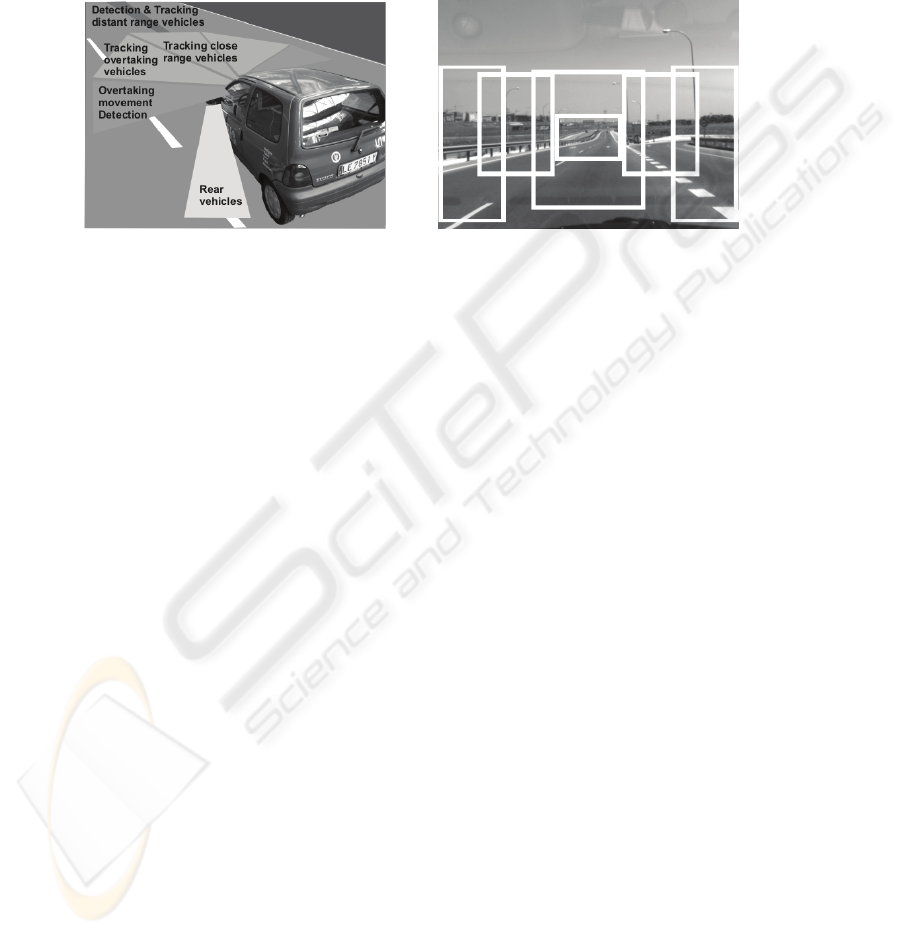
2 Different Areas and Vehicle Appearance
Different features define the same vehicle depending on the area of the image where
it appears. As it is shown in Fig. 1, lateral areas of the images are the only ones where
overtaking vehicles can appear. Depending on the country, overtaking vehicles will
appear on the left/right lane, and overtaken vehicles on the right/left one. A model-
based approach is difficult to implement and it is better to use a feature-based ap-
proach, mainly taking movement into account. A different case is when the vehicle is
in front of the camera. The rear part of the vehicle is full seen in the image and a
model-based approach is possible. Beside these areas, there is another corresponding
to the vehicles have just over-taken ours. The rear part of the vehicle is completely
seen in the image, although a small deformation due to projective distortion appears.
58
It will be shown that the same model-approach can be applied. The vehicles can ap-
pear from the laterals of the image and from a far distance. Depending on which case
one detector or another is chosen. Then the vehicle trajectory has to be tracked until it
is out of sight.
3 Detection of Overtaking Vehicles
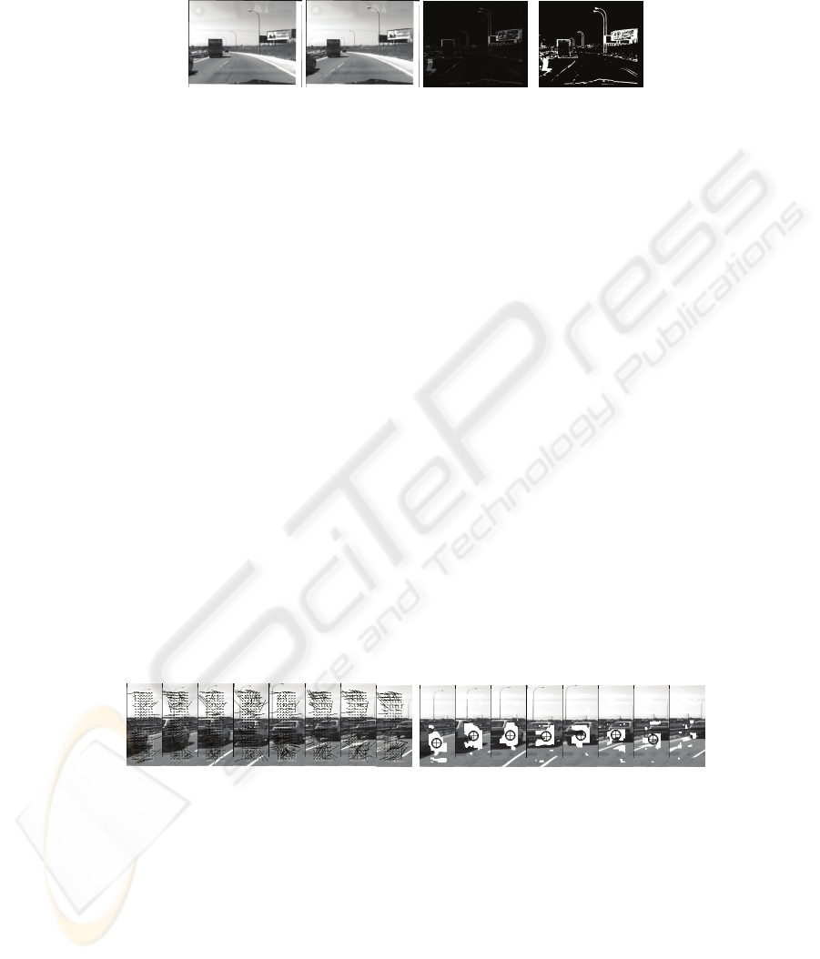
Mainly, there are three approaches to detect overtaking vehicles: Image difference,
learning from examples and optical flow. Image difference [6] has the main advan-
tages of simplicity and speed and its basics is the lack of texture in the objects sur-
rounding the vehicle. The main drawbacks are the little information (magnitude, ori-
entation) of the movement, and, that the effect of the shock absorbers, the presence of
guardrails and a textured environment can cause the same result as an overtaking car.
To show this, the absolute value of image difference is shown in Fig. 2.b and the
binary images in Fig. 2.c. There is no threshold able to eliminate the background and
only filter the vehicle. An example of NN-based movement detection is [10], where
an algorithm based on a Time Delay NN with spatio-temporal receptive fields was
proposed for detecting overtaking vehicles. It does not provide information about the
range and direction of the movement.
That is why some authors have preferred optical flow, as the movement can be fil-
tered taking into account its range and direction. In [11] they use a planar parallax
model to predict where image edges will be looked for after travelling a certain dis-
tance. Detection of overtaking vehicles given the vehicle velocity and camera calibra-
tion is done in [12]. The image motion is obtained and image intensity of the back-
ground scene is predicted. A difference with the methods above is the need of ego-
motion estimation while in our case it is not necessary because the vehicle is going to
be tracked.
Movement
Detection
Movement
Detection
Distant
Vehicles
Close vehicles
Overtaking
vehicles
Overtaking
vehicles
(a) (b)
Fig. 1. Image areas and vehicle appearance.
59
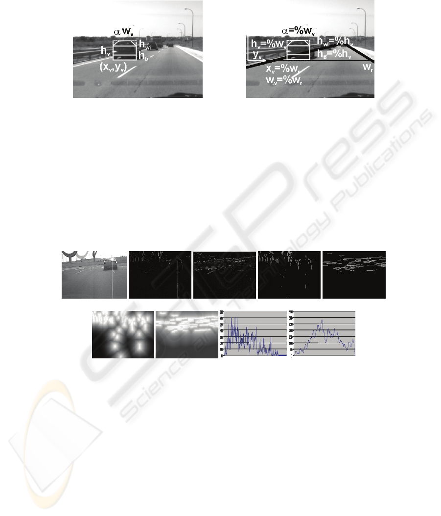
There are several methods to obtain optical flow. In this paper, block similarity has
been used due to the movement range. The similarity is obtained through the sum of
absolute differences because it is a good deal between speed and accuracy. In Fig. 3
there is a detection of the overtaking car. Its movement is filter based on three fea-
tures: range, direction, and size of the blobs with the same movement. Range is useful
to discriminate fast movements against false movements produced by noise. Direction
is useful to discriminate overtaking vehicles against any other object that it is over-
taken by our vehicle. In order to speed up the algorithm, this is done only for those
pixels whose difference with the previous images is bigger than a threshold. There-
fore a thresholding is done if:
⎪
⎪
⎩
⎪
⎪
⎨
⎧
⎪
⎩
⎪
⎨
⎧
≥
≤≤
≤≤
=
elsewhere0
),,,(
),(
S),(S
1
),(
21
maxmin
A
TjiyxSAD
yx
yxR
yxI
θθθ
(1)
The blobs are detected, and if one of them is greater than an area threshold there is
an overtaking vehicle (Fig. 3-b). When the vehicle is no longer detected, the tracking
module (described later) is called and it receives the information of the vehicle posi-
tion in order to track it using a geometric model. A similar reasoning is used detecting
when our vehicle is overtaking another; the tracking module will call the movement
based detection module, as the geometric information is no longer useful.
(a) (b) (c)
Fig. 2. Movement detection based on image difference. (a) Image sequence (b) Absolute
value of image differences (c) thresholding of the previous images.
(a) (b)
Fig. 3. Detection of overtaking vehicles. (a) Optical flow detection (b) Thresholding and blob
analysis.
60
4 Distance Measurement Error due to Camera Coordinates
Stein et al. [13] demonstrated how an ACC could be based on a monocular vision
system. Their implementation was the simplest one: the world is flat and the camera’s
optical axe is parallel to the road. This configuration has the main disadvantage that
one object at the farthest distance projects itself at the middle height of the image.
This way half of the sensor is useless to obtain distances. In our case the camera is
looking slightly to the ground instead of the front. Then, in order to obtain the dis-
tance Y of the object located with coordinates (u,v):
θθ
θ
θ
cossin
sincos
vf
vf
hY
−
+
=
θθ
θ
θ
sincos
cossin
hY
hY
fv
+
−
=
(2)
Where
θ
is the angle of the optical axe with the horizontal plane, h is the height of
the camera and
f is the focal length. These parameters can be calculated through a
calibration algorithm [14].
If an error of
δ
±
pixels is supposed, the true distance is between the ranges:
()
θδθθ
δ
22
2
coscossin
2
−−
=Δ
vf
fh
Y
(3)
And, the relationship with distance is:
(
)
Y
hY
fhY
Y
2
sincos
2
θθ
δ
+
≈
Δ
(4)
Because
() ( )
22
cos
θδ
>>fh .
The most important conclusion is that the distance range and its relationship with
respect the distance, obtained from (3) and (4), are independent of the camera incline
for short and medium distances. This way, for vehicles at less than 200 meter the
values are nearly the same. This agrees with [13], where the formula is (following our
notation):
Y
fhY
Y
δ
2
≈
Δ
(5)
And, for some typical values is:
Y
Y
Y
10 2.263
3-
=
Δ
(6)
While, in our case, the data obtained through Least Squares are:
⎪
⎪
⎩
⎪
⎪
⎨
⎧
=≈+
=≈+
=≈
=
Δ
º10 10 2.24710 .74 10 2.247
º5 10 2.28810 .80 10 2.288
º0 10 2.27910 1.4- 10 2.279
3-4-3-
3-4-3-
-3-4-3
θ
θ
θ
YY
YY
YY
Y
Y
(
7)
61
That is, experimentally it is shown for certain angles
θ
θ
sincos hYY >>
≈
and
therefore equations (4) and (5) are equivalent. It is known that the main source of
error is the incline of the camera that, although can be calibrated in advanced, suffers
from mechanical vibrations or the shock absorbers effect. In order to correct the error,
the real angle is obtained computing the vanishing point after the road has been de-
tected. Therefore equation (6) is used for the tracking process as an indicator of the
accuracy of detection and it can be used for the error covariance of the measurement
equation.
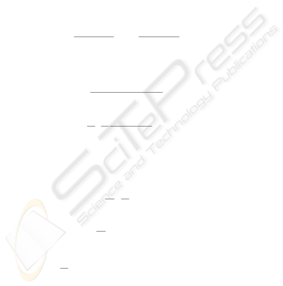
5 Geometric Models
Due to shadows, occlusions, weather conditions, etc., the model has to incorporate as
much information as possible. In [15], a vehicle was defined by seven parameters
(Fig. 4): position (x,y), width and height of the vehicle, windshield position, bumper
position and roof angle. As the road is previously detected, the y coordinate of the
vehicle provides its distance and the rest of the values can be geometrically coherent.
Some functions were calculated from the image to enhance three features that define
(a) (b)
Fig. 4. Geometric model of a vehicle. (a) the seven parameters (b) The values of theses pa-
rameters are constrained by the detection of the road.
(a) (b) (c) (d) (e)
(f) (g) (h) (i)
Fig. 5. (a) Image (b) Vertical and (c) horizontal gradient (d) Vertical and (e) horizontal edges
(f) vertical and (g) horizontal distances (h) vertical and (i) horizontal symmetries.
62

a vehicle (Fig. 5): symmetry: the vertical and horizontal edges of the image were
found and the vertical symmetry axis calculated; shape: defined by two terms, one
based on the gradient and the other one based on the distance to the edges found
before; vehicle shadow: defined by the darkest areas in the image. The searching
algorithm for the correct values of the model was based on Genetic Algorithms (GAs)
due to their ability to reach a global maximum surrounded by local ones.
6 Perceiving the Environment
The detection and tracking of vehicles is done for multiple resolutions. A Gaussian
pyramid is created. The information of the detection of lower and greater levels is
mutually exchanged. Working under a multi-resolution approach has the main advan-
tage of choosing the best resolution for every circumstance. For example, the number
of individuals in the GA needed to find the vehicles can be different. As the resolu-
tion is greater the number of individuals needed grows. It is worthwhile noticing that
the low resolution number of individuals has been reduced because overtaking detec-
tion module information has been taken into account, Fig. 6-a. This way the range of
the y value of the geometric model is limited between the lowest y value of the blob
detected and its centre of gravity. Finally, tracking the vehicle (Fig. 6-b) also reduces
the number of individuals as they are distributed around the best individual of the
previous image. The values are shown in Table 1.
Two options for the tracking of the vehicles have been studied. The first one is
based on GA. A prediction of the position of the vehicle is performed taking into
account the previous image and the speed. The population is initialized around that
value. The second approach is a Kalman Filter where the measure error is modelled
by equation (6).
Table 1. Number of individuals depending on the resolution and tracking or not the vehicle.
Generations Population
Minimum resolution (no tracking) 2 64
Medium resolution (no tracking) 2 64
Maximum resolution (no tracking) 40 128
Minimum resolution (tracking) 2 32
Medium resolution (tracking) 2 32
Maximum resolution (tracking) 10 64
63
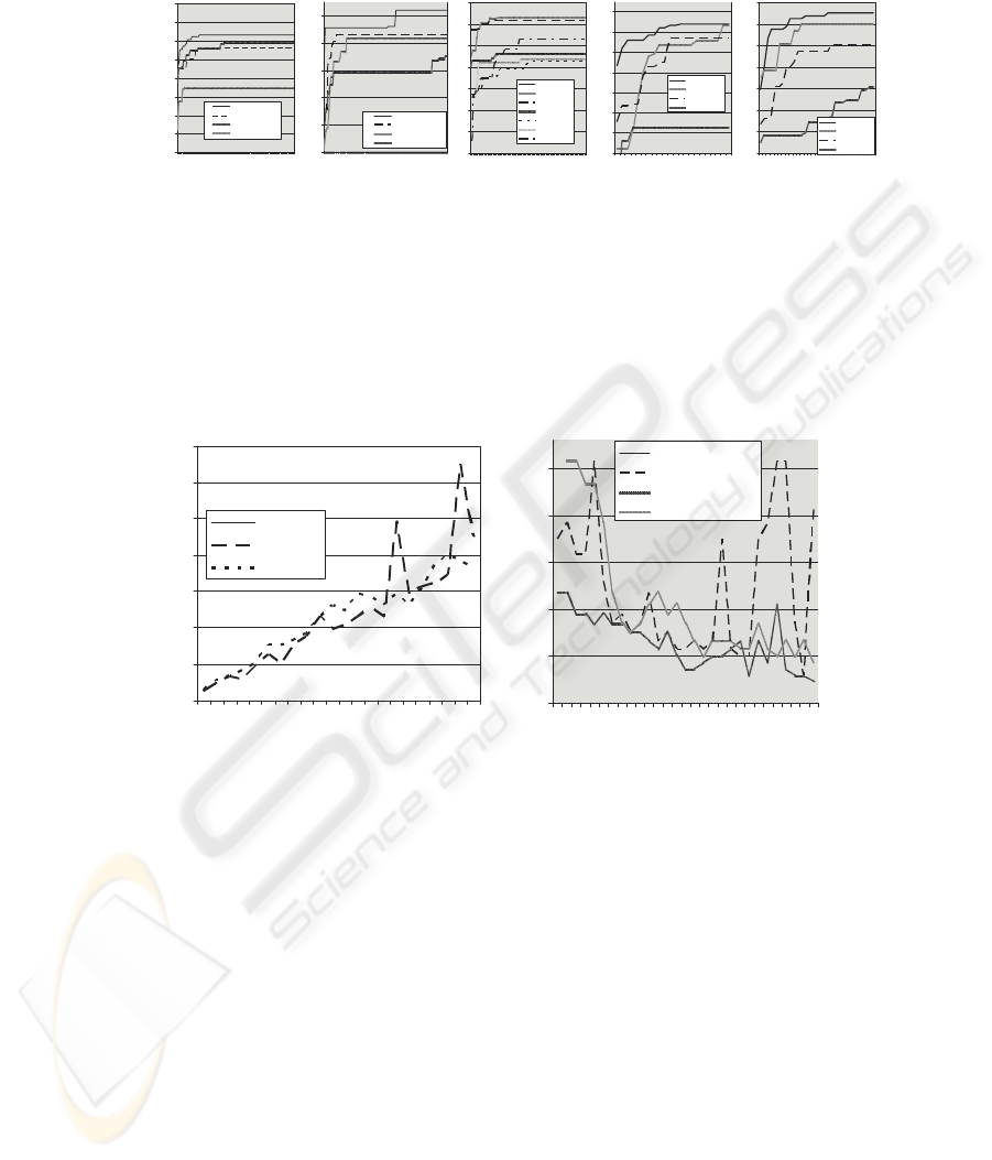
The two results are compared, in Fig. 7, with the ones obtained manually and with
no time integration. Two cases are considered: tracking an overtaking vehicle and the
detection and tracking of a slower vehicle. For the first case the Kalman filter predicts
a position of the vehicle form the previous position and speed estimation. This predic-
tion is passed to the model parameters space and the individuals of the GA are initial-
ized around that value. The deviation depends on the covariance matrix following the
σ
3 rule. Once the GA finishes, the best individual solution is given to the medium
level and when it is finished, to the maximum resolution one. This final result is used
for the correction step of the Kalman filter. The second case, tracking of a slower
vehicle, is performed in the image at maximum resolution for large distances. The GA
works until a maximum number of iterations is reached or it converges to a value
higher than a threshold. If it is the first case, it is concluded there is no vehicle an a
new image is grabbed and if it is the second case, the tracking of the vehicle starts.
Some examples are shown in Fig. 8. In the overtaking detection, the algorithm is
able to refine the values and correct a small error in width at low resolution. Kalman
tracking gives better results against the GA tracking as the prediction is better. In Fig.
8-d the algorithm detects a new vehicle appearing in the image with a better fitness
while Kalman still tracks the old one.
500
550
600
650
700
750
800
850
900
1 21416181101121
Iteration
F
i
t
n
e
s
s
16 Individuals
8 Individuals
16 Individuals (II)
8 Individuals (II)
Fitne ss
740
760
780
800
820
840
121416181101121
Iteration
64 Individuals
32 Individuals
64 Individuals (II)
32 Individuals (II)
680
700
720
740
760
780
800
82
0
1 4 7 1013161922252831
Iteration
Fitness
128 Individual s
64 Individuals
32 Individuals
16 Individuals
Maximun Resolution
800
820
840
860
880
900
920
940
1 3 5 7 9 11 13 15 17 19 21
Iteration
Fitness
128 Indiv iduals
64 Individual s
32 Individual s
16 Individual s
Medium Resolution
500
550
600
650
700
750
800
850
1 7 13 19 2 5 31 37 43 49 55 61 67 73 79
Iter ation
Fi
t
n
e
s
s
128 Individuals
64 Individual s
32 Individual s
16 Individual s
8 Individuals
4 Individuals
2 Individuals
(a) (b)
Fig. 6. Number of individuals needed for every resolution (a) when the overtaking informa-
tion is taking or not into account (b) if tracking is performed.
Vehicle detection
10,00
20,00
30,00
40,00
50,00
60,00
70,00
80,00
1 3 5 7 9 111315171921
Frame
Di
s
tan
c
e
(
m
)
Mannually
GA
Kalman
20,00
25,00
30,00
35,00
40,00
45,00
1 4 7 10131619222528
Frame
s
D
i
s
t
a
n
c
e
(
m
)
Mannually
GA no prediction
GA prediction
Kalman
(a) (b)
Fig. 7. Detection and tracking of (a) Overtaking vehicle (b) Approaching vehicle.
64
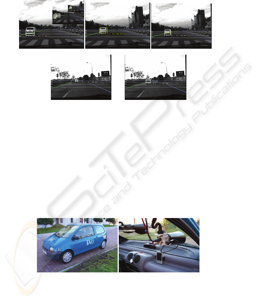
7 Conclusions
A system based on computer vision for the detection of surroundings vehicles has
been presented in this paper. Experiments were carried out in the IVVI (Intelligent
Vehicle based on Visual Information) vehicle (Fig. 9), which is an experimentation
platform for researching and developing Advance Driver Assistant Systems based on
Image Analysis and Computer Vision. There are two PCs in the vehicle's boot for
image analysis from a stereo vision system and a colour camera. The position and
speed of the vehicle is provided by a GPS connected through a Bluetooth link to a
PDA, which broadcast this information to the PCs by a WiFi Network.
(a) (b) (c)
(d) (e)
Fig. 8. (a) Pyramidal overtaking detection (b) GA tracking (c) Kalman tracking (d) GA detec-
tion (e) Kalman tracking.
(a) (b)
Fig. 9. IVVI Vehicle. (a) Experimental Vehicle (b) stereo and color camera.
65

Acknowledgements
This work was supported in part by the Spanish Government under Grant TRA2004-
07441-C03-01.
References
1. H. Mori, N. M. Charkari, and T. Matsushita, On-line vehicle and pedestrian detections
based on sign pattern, IEEE Trans. on Industrial Electronics, vol 41, pp. 384-391, 1994.
2. T. Zielke, M. Brauckmann, and W. Von Seelen, Intensity and edge-based symmetry detec-
tion with application to car-following, CVGIP: Image Understanding, vol. 58, pp. 177-190,
1993.
3. C. Goerick, D. Noll, and M. Werner, Artificial Neural Networks in Real Time Car detec-
tion and Tracking Applications, Pattern Recognition Letters, vol. 17, pp. 335-343, 1996.
4. T.K. ten Kate, M.B. van Leewen, S.E. Moro-Ellenberger, B.J.F. Driessen, A.H.G. Versluis,
and F.C.A. Groen, Mid-range and Distant Vehicle Detection with a Mobile Camera, IEEE
Intelligent Vehicles Symp. 2004
5. Broggi, P. Cerri, and P.C. Antonello, Multi-Resolution Vehicle Detection using Artificial
Vision, IEEE Intelligent Vehicles Symp. 2004.
6. M. Betke, E. Haritaoglu, and L.S. Davis, Real-time multiple vehicle detection and tracking
from a moving vehicle, Machine Vision and Applications, vol. 12, pp. 69-83, 2000.
7. JM. Ferryman, S.J. Maybank, and A.D. Worrall, Visual surveillance for moving vehicles,
International Journal of Computer Vision, vol. 37, pp. 187-97, 2000
8. T. Kato, Y. Ninomiya, and I. Masaki, Preceding vehicle recognition based on learning from
sample images, IEEE Trans. on Intelligent Transportation Systems, vol. 3, pp. 252-260,
2002.
9. Z. Sun, G. Bebis, and R. Miller, On-Road Vehicle Detection Using Optical Sensors: A
Review, IEEE Intelligent Transportation Systems Conf. 2004.
10. Wohler, and J.K. Anlauf, Real-time object recognition on image sequences with adaptable
time delay neural network algorithm-applications for autonomous vehicles, Image and Vi-
sion Computing, vol. 19, pp. 593-618, 2001.
11. P. Batavia, D. Pomerleau, and C. Thorpe, Overtaking Vehicle Detection Using Implicit
Optical Flow, IEEE Transportation Systems Conf. 1997.
12. Y. Zu, D. Comaniciu, M. Pellkofer, and and T. Koehler, Passing Vehicle Detection from
Dynamic Background Using Robust information Fusion, IEEE Intelligent Transportation
Systems Conf. 2004.
13. G. Stein, O. Mano, and A. Shashua, Vision-based ACC with a Single Camera: bounds on
Range and Range Rate Accuracy, IEEE Intelligent Vehicles Symp. 2003.
14. J. M. Collado, C. Hilario, A. De la Escalera, J.M. Armingol. Self-calibration of an On-
Board Stereo-Vision System for Driver Assistance Systems, IEEE Intelligent Vehicle
Symp. 2006.
15. Hilario, J. M. Collado, J. Mª Armingol,A. de la Escalera, Pyramidal Image Analysis for
Vehicle Detection, IEEE Intelligent Vehicles Symp. 2005.
66
