
IMAGE DECONVOLUTION USING A STOCHASTIC
DIFFERENTIAL EQUATION APPROACH
∗
X. Descombes
1
, M. Lebellego
1,2
1
Ariana Research Group, INRIA/I3S, 2004, route des lucioles, BP 93, 06902, Sophia Antipolis Cedex, France
E. Zhizhina
2
2
Dobrushin Laboratory, IITP of RAS, Bol’shoi Karetnyi per., 19, 127994, GSP-4, Moscow, Russia
Keywords:
Image deconvolution, Stochastic Differential Equation, Langevin dynamics, Euler approximation.
Abstract:
We consider the problem of image deconvolution. We foccus on a Bayesian approach which consists of
maximizing an energy obtained by a Markov Random Field modeling. MRFs are classically optimized by a
MCMC sampler embeded into a simulated annealing scheme. In a previous work, we have shown that, in the
context of image denoising, a diffusion process can outperform the MCMC approach in term of computational
time. Herein, we extend this approach to the case of deconvolution. We first study the case where the kernel
is known. Then, we address the myopic and blind deconvolutions.
1 INTRODUCTION AND
METHOD
Image restoration is a wellknown ill-posed problem
which has motivated many works. A first complete re-
view of image restoration approaches was given (An-
drews and Hunt, 1977). Since then, numerous ap-
proacheshave been proposed, among them variational
and stochastic approaches play a leading role. How-
ever, there is still no completly satisfactory solution,
especially in case of blind deconvolution, for which
the kernel is unknown. As an ill-posed problem,
image restoration is adapted to Bayesian approaches
which embed a prior model, which constrains the so-
lution. Therefore, models based on Markov Random
Fields (MRFs), preserving the discontinuities while
restoring the data have been proposed (Geman and
Reynolds, 1992). More sophisticated Markov mod-
els have been recently proposed, such as in (Molina
et al., 2000; Mignotte, 2006). Classically, MRFs, for
image restoration, are optimized using a Gibbs sam-
pler embedded in a simulated annealing scheme (Ge-
man and Geman, 1984). In this paper, we consider a
classical MRF modelling but explore a new optimiza-
tion scheme based on a stochastic differential equa-
∗
The authors would like to thank EGIDE for partial fi-
nancial support within the ECONET project 10203YK.
tion approach. In a previous work, we have shown
that this new scheme outperforms the Gibbs sampler
in term of computational time in the case of image de-
noising (Descombes and Zhizhina, 2004). We extend
this work to the deconvolution problem.
1.1 The Stochastic Approach for Image
Deconvolution
We consider a degraded image Y. The degradation,
including noise and blurring can be modelled by the
following equation :
Y = K ∗ X + n (1)
Where X is the original image without noise, that we
want to reconstruct, n is a Gaussian additive noise
and K a convolution kernel.
Then the different steps of this approach are the
following :
• We define an energy function associated to a con-
figuration X
• We construct a diffusion process based on this en-
ergy thanks to the Langevin operator
• We derive from this process a discretized process
for computer simulations.
157
Descombes X., Lebellego M. and Zhizhina E. (2007).
IMAGE DECONVOLUTION USING A STOCHASTIC DIFFERENTIAL EQUATION APPROACH.
In Proceedings of the Second International Conference on Computer Vision Theory and Applications, pages 157-164
DOI: 10.5220/0002064701570164
Copyright
c
SciTePress

• We finally define an estimator to optimize the
model and find a solution
1.2 Energy Function
To the configurations X, we associate an energy func-
tion, which is interpreted as the Hamiltonian of a
Gibbs field.
The energy is defined by the sum of an interac-
tion term, modelling some prior knowledge and a data
driven term:
H(X,Y) = Φ
1
(X) + Φ
2
(X,Y) (2)
with
Φ
1
(X) = β ·
∑
(i, j)∈Λ, j∈V(i)
U(X
i
− X
j
) (3)
and
Φ
2
(X,Y) = λ ·
∑
i
((K ∗ X)(i) −Y
i
)
2
(4)
Where Λ is the set of all the pixels in the image. And
V(i) is the neighborhood of the pixel i. λ and β are
two parameters of the model. β controls the smooth-
ness and λ the weight of the data.
The function U is the following :
U(X
i
− X
j
) = −
1
1+
(X
i
−X
j
)
2
d
2
(5)
U is a φ-function, as proposed in (Geman and
Reynolds, 1992), d is a parameter. The bigger d, the
smoother the image.
1.3 The Langevin Equation
We then want to construct a diffusion process :
X(t) = {X
i
(t) ∈ [0, 512], i ∈ Λ}
on the configuration space E = [0, 512]
|Λ|
, which is
a stationary Markov process with the Gibbs measure
associated with the above Hamiltonian H(X,Y) :
dµ
σ
=
e
−
2
σ
2
·H(X,Y)
Z
σ
· dµ
σ
(6)
To construct this process, we consider the func-
tional Hilbert space L
2
(E, dµ
σ
)
Let’s us consider the operator L
f
defined on the func-
tion space E by the following equation :
L
σ
f · dµ
σ
=0 (7)
where dµ
σ
is the Gibbs measure. It is a generator of
the stationary process with the invariant measure µ
σ
.
It is a generator of a Langevin dynamics. There is not
a unique solution of the equation (6), but the follow-
ing generator is one of them :
L
σ
f =
1
2
· σ
2
· ∆f − ∇H · ∇f
=
1
2
· σ
2
·
∑
i∈Λ
∂
2
f
∂x
2
i
−
∑
i∈Λ
∂H
∂x
i
·
∂f
∂x
i
(8)
This generator is a generator of a diffusion process.
We now have an operator defined on the functional
space. From this process on the functional space, it is
possible to reconstruct the process on the configura-
tion space.
Using the relation between the two processes, we
get the following stochastic equation, describing the
evolution of the configuration :
dX(t) = σ· dW(t)
|
{z }
I
−∇
X
H(X,Y) · dt
|
{z }
II
(9)
The second term of this equation (II), is a deter-
ministic term, depending on the gradient of the energy
function. The first term of this equation (I), is a diffu-
sive term, W = {W(t), t ≥ 0} being a m-dimensional
Wiener process. So this equation can be interprated
as a gradient descent with a random part, σ being the
temperature of the scheme.
Since the stochastic equation describes the station-
ary process, the realization of X(t) at time t will be a
typical configuration of the Gibbs measure dµ
σ
.
1.4 The Euler Approximation
In section 1.3, we have constructed a continuous
process. But we need to discretize it to perform com-
puter simulations. Therefore, we consider an approx-
imation of the process by a discrete time Markov
process.
To discretize the process, we use the Euler ap-
proximation (Kloeden and Platen, 1992). We con-
sider a time discretization of the interval [0, t]: τ(δ) =
{τ
n
, n = 0..n
t
} by time steps δ
n
= τ
n+1
− τ
n
The approximation process Z(n) = { Z
i
(n), i ∈ Λ},
n = 0..n
t
has the same initial state X(0) as the
process X(t), and can be constructed by the following
iterative scheme :
VISAPP 2007 - International Conference on Computer Vision Theory and Applications
158
Z
i
(0) = X
i
(0)
Z
i
(n+ 1) = Z
i
(n) + a
i
(Z(n),Y) · δ
n
+
σ· (W(τ
n+1
) −W(τ
n
))
(10)
Where a
i
(Z
n
,Y) = −∇
i
H(Z(n),Y) and σ · dW is a
Wiener process. In practice, W(τ
n+1
) − W(τ
n
) can
be simulated by sampling a centered normal law
N (0, δ
n
) with a variance equal to δ
n
.
1.5 The Estimator
Finally, we define an estimator which optimizes the
Hamiltonian. We use here the Maximum A Posteri-
ori (MAP) criterion. The MAP criterion consists in
minimizing the energy H :
ˆ
X= argmin
X
H(X,Y)
So we are looking for a configuration X giving the
global minimum of the Hamiltonian. To estimate
ˆ
X , we apply a simulated annealing scheme where
the temperature parameter σ decreases during itera-
tions.We also make decrease the time discretization
parameter of the equation (10) : δ
n
.
In theory to avoid local minima, the decreasing
scheme of the parameter σ have to be logarithmic. In
practice, for some computational reasons , we con-
sider an exponential decreasing scheme for both pa-
rameters : e
α·t
but with α close to zero. For the tests,
we have considered σ decreasing from 1 to 0.01 and
between 1000 and 3000.
1.6 Results with a Known Kernel
We first consider that the convolution kernel K is
known. That means we know exactly the blur of the
picture, which is of course a strong constraint. The
second step will be to consider that we don’t know
this kernel.
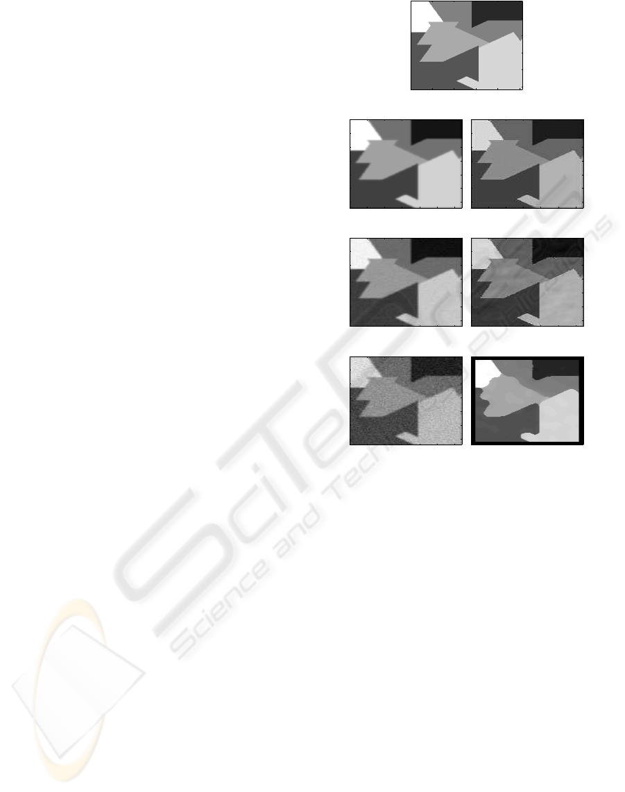
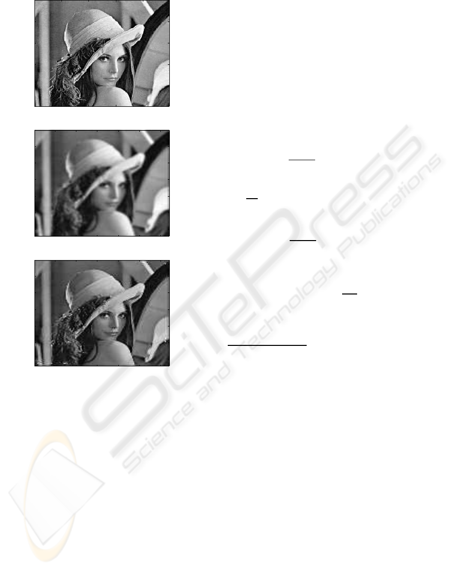
The simulations for the different algorithms have
been done on two different 128x128 images : a syn-
thetic image consisting of several uniform areas (see
figure 1) and Lena picture (see figure 2), which were
blurred by a 7x7 Kernel, and on which we have added
a centered Gaussian noise (with different standard de-
viations s). Here, we assume that we know exactly the
convolution kernel. Results on the synthetic image for
s = 0, 3, 10 are shown on figure 1 for the synthetic im-
age and on figure 2 for Lena picture.
For high level of noise (s = 10), we have to con-
sider a stronger prior (high value for parameter β)
which leads to an edge delocalization.
50 100 150 200 250
50
100
150
200
250
ORIGINAL IMAGE
20 40 60 80 100 120
20
40
60
80
100
120
20 40 60 80 100 120
20
40
60
80
100
120
BLURRED IMAGE s = 0 DECONVOLVED IMAGE
20 40 60 80 100 120
20
40
60
80
100
120
20 40 60 80 100 120
20
40
60
80
100
120
BLURRED IMAGE s = 3 DECONVOLVED IMAGE
20 40 60 80 100 120
20
40
60
80
100
120
20 40 60 80 100 120
20
40
60
80
100
120
BLURRED IMAGE s = 10 DECONVOLVED IMAGE
Figure 1: Deconvolution for s = 0, 3, 10.
In practice, we rarely have any information about
the kernel. So let’s now consider the case where the
kernel is unknown. We then have to estimate its co-
efficients or to introduce a parametric model for the
kernel.
2 BLIND DECONVOLUTION
2.1 A Stochastic Scheme for K
In this second scheme, we have two unknowns to up-
date at each iteration: the current image X and the
kernel K.
The stochastic scheme for X is :
X
i
(n+ 1) = X
i
(n) + a
i
(X(n), K(n),Y)· δ
n
1
+ σ
1
·
(W(τ
n+1
) −W(τ
n
))
Where a
i
(X(n), K,Y) = −∇
X
i
H(X(n), K,Y)
And we now introduce a stochastic scheme for K :
IMAGE DECONVOLUTION USING A STOCHASTIC DIFFERENTIAL EQUATION APPROACH
159
50 100 150 200
50
100
150
200
ORIGINAL IMAGE
20 40 60 80 100 120
20
40
60
80
100
120
BLURRED IMAGE
20 40 60 80 100 120
20
40
60
80
100
120
RECOVERED IMAGE
Figure 2: Deconvolution for s = 1.
K
i
(n+ 1) = K
i
(n) + b
i
(X(n), K(n),Y)· δ
n
2
+ σ
2
· (W(τ
n+1
) −W(τ
n
)) (11)
Where b
i
(X, K,Y) = −∇
K
i
H(X, K,Y)
Prior Knowledge on K
Here we do not want to introduce a strong prior
knowledge on K, because we assume we don’t know
anything on K. But still, we want it to be a convolu-
tion kernel, so it has to be normalized. But this prior
knowledge doesn’t play any role in the energy func-
tion. We don’t introduce it in the prior term but just
normalize the kernel at the end of each iteration.
We thus suppose, if we denote K = (k
s
) , that
∑
s
k
s
=1
K Dynamics
The energy function is : H(X, K,Y) = λ
1
·φ
1
(X)+λ
2
·
φ
2
(X, K,Y)
φ
1
is the prior knowledge term, φ
2
is the data-attached
term. And :
φ
2
(X, K,Y) =
∑
i, j
(K ∗ X
i, j
−Y
i, j
)
2
=
∑
i, j
∑
u=(v,w)
k
v
· X
i+v−N, j+w−N
−Y
i, j
2
(12)
Where :
u = v· dimK + w, w < dimK
N =
dimK−1
2
So the derivative of the energy w.r.t. k
s
is :
∂φ
2
∂k
s
= 2·
∑
i, j
X
i+a−N, j+b−N
(K ∗ X(i, j) −Y
i, j
)
Where :
s = a · dimK+ b, b < dimK
N =
dimK−1
2
And finally
b
i
(X, K,Y) = −λ
2
·
∂φ
2
∂k
i
(13)
= −2·λ
2
·
∑
i, j
X
i+a−N, j+b−N
(K ∗ X(i, j) −Y
i, j
)
Scheme Parameters
Let’s come back to the new stochastic scheme:
K
i
(n + 1) = K
i
(n) + b
i
(X(n), K(n),Y) · δ
n
2
+ σ
2
·
(W(τ
n+1
) −W(τ
n
))
We can suppose that this second scheme has no
connection with the first one: the variations of X
i
and
k
s
at each iteration are not of the same order. So
we have different coefficients δ and σ for the two
schemes.
Again we choosed a normal law for the probabilis-
tic part. Here k
s
belongs to [0, 1]. So the more intuitive
is to take again a normal law centered on 0. So that
we have a high probability not to move far.
Update of X and K
We can then wonder about the order of updating of
the two unknowns. We have two possibilities :
1. At each iteration I of the scheme, we update X and
then K
2. We make N iterations for X and then M for K and
then we come back to X with the new K and so on
···
VISAPP 2007 - International Conference on Computer Vision Theory and Applications
160
Each one has drawbacks :
In the first one, we recalculate the Kernel after each
iteration of X. But at each iteration, there are only
slight changes on X. And so the recalculation of the
kernel at each steps does not take into account enough
changes. In the second one, let’s suppose we have
a poor estimate of the kernel in the current configu-
raiton. Then, making a big number of iterations on X
degrades it strongly, and then the next calculation on
the kernel will be even worse. So each new update de-
grades more the picture. In such a case, to convergeto
the MAP would require a very low decreasing scheme
for the parameters δ and σ. In practice we choose the
second scheme but with moderate values for N and
M.
As we have now introduced a new scheme and
new calculations of the derivatives, the computational
time required to obtain the convergence will be highly
increased. However, here we have a possibility to
minimize the time of calculation: instead of calculat-
ing the parametric kernel with information from the
entire image, a little window in the image is used to
find out the informationto evaluate the Kernel. This is
possible because we assumed that the blur is uniform
on the image. This window can be chosen randomly
in the image or can be fixed at the beginning of the
algorithm. But we have to be careful in the choice of
this window, because if we pick up an homogeneous
part of the image, without any information on edges,
this window will not contain any information on the
blur. So the evaluation of the kernel will not be accu-
rate.
2.2 Results
The introduction of the convolution product into the
derivative of the of φ
2
has brought a first difficulty.
The problem with this derivative
∂φ
2
∂k
s
= 2·
∑
i, j
X
i+a−N, j+b−N
(K ∗ X(i, j) −Y
i, j
)
is that the value is very big. In fact, it is a sum on
all the pixels of the image and each term has a high
value, negative or positive.
Consequently we had to ponderate this term so
that we don’t have too big steps between the former
coefficient of K and the new one. But if we introduce
a very small coefficient λ
2
it will also affect the sto-
chastic scheme for X. And as the derivative of φ
2
is
not that high w.r.t X
i
, the attach to the data will not
be strong enough. We introduced a coefficient which
ponderates this derivative but only in the stochastic
scheme concerning K. This coefficient is quite large
and depends on the size of the image. The bigger the
image, the bigger this coefficient.
20 40 60 80 100 120
20
40
60
80
100
120
20 40 60 80 100 120
20
40
60
80
100
120
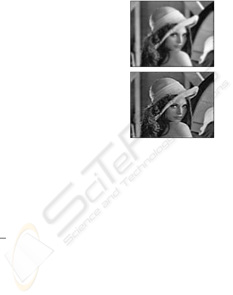
Figure 3: Blurred image (top), Recovered after 4000 itera-
tions (bottom).
The initialization have been made to the identity
Kernel. During the first iterations, the algorithm tends
to the right solution. For example, the result on fig-
ure 3 is obtained with 4000 iterations on the blurred
Lena Picture. However, if we run the algorithm up to
the convergence, we obtained an uniform kernel. We
therefore have to constrain the problem by adding a
prior on the kernel to avoid this trivial solution.
3 MYOPIC DECONVOLUTION
As seen in the previous section , the blind deconvolu-
tion is quite complex and the convergence is not ob-
tained. We now introduce a prior knowledge on the
convolution kernel K. In this section, we develop an
algorithm dealing with a parametric model of the ker-
nel (which represents a Gaussian blur in our case).
3.1 Gaussian Kernel
Modelling As we supposed we have a Gaussian
Blur, the kernel can be written as :
IMAGE DECONVOLUTION USING A STOCHASTIC DIFFERENTIAL EQUATION APPROACH
161

K
i, j
=
1
Z
· e
−
k×
(
(i−c)
2
+( j−c)
2
)
(14)
Where :
c =
dimH− 1
2
is the coordinate of the center
1
Z
is a normalization term
k is twice the inverse of the variance
Here the prior knowledge, is not introduced in the
energy function, like for the image, but in the fact
that we now only consider a single parameter k and
that we impose a Gaussian shape for the kernel.
This model has the following advantage: we have
an unique unknown, k =
1
σ
2
, to estimate instead of
the 49 unknowns in the blind deconvolution.
We have to calculate the new derivative of the
energy function. The energy has not changed:
H(X,Y, K) = λ
1
·ϕ
1
(X) + λ
2
·φ
2
(X, K,Y) where now:
φ
2
(X, K,Y) =
∑
i, j
(K ∗ X
i, j
−Y
i, j
)
2
(15)
=
∑
i, j
∑
(a,b)
k
a,b
· X
i+a−N, j+b−N
−Y
i, j
!
2
=
∑
i, j
∑
(a,b)
1
Z
· e
−k{(a−N)
2
+(b−N)
2
}
·X
i+a−N, j+b−N
−Y
i, j
2
And where : N =
dimK−1
2
. Let us then write the
derivative of φ
2
:
∂φ
2
∂k
s
= 2·
∑
i, j
∑
a,b
(
1
Z
· e
−kA
· X
i+a−N, j+b−N
−Y
i, j
)
×
∑
a,b
−1
Z
· A·e
−kA
· X
i+a−N, j+b−N
−Y
i, j
(16)
where A = (a− N)
2
+ (b− N)
2
.
which can be written as:
∂φ
2
∂k
s
= 2·
∑
i, j
K ∗ X(i, j) −Y
i, j
· (17)
∑
a,b
(
−1
Z
· A·e
−kA
· X
i+a−N, j+b−N
−Y
i, j
Here we suppose that the factor
1
Z
does not depend
on k. This is a first approximation because in fact:
1
Z
=
q
k
2·π
Results The considered kernel is the following:
K=
0 0 0 0.01 0 0 0
0 0 0.01 0.02 0.01 0 0
0 0.01 0.05 0.1 0.05 0.01 0
0.01 0.02 0.1 0.2 0.1 0.02 0.01
0 0.01 0.05 0.1 0.05 0.01 0
0 0 0.01 0.02 0.01 0 0
0 0 0 0.01 0 0 0
It is not exactly a gaussian Kernel. The following
matrix is the gaussian matrix obtained for k = 1.6 :
K=
0 0 0 0 0 0 0
0 0.001 0.009 0.016 0.009 0.001 0
0 0.009 0.057 0.106 0.057 0.009 0
0 0.016 0.106 0.198 0.0106 0.016 0
0 0.009 0.057 0.106 0.057 0.009 0
0 0.001 0.009 0.016 0.009 0.001 0
0 0 0 0 0 0 0
To face again the problem of huge derivative of φ
2
, as seen above, we have introduced a dividing fac-
tor, but also we constrain k to belong to the interval
[0.1;3].
Results of the simulations: Despite of these
measures, we still have problem with the φ
2
deriva-
tive:
Through this Gaussian form, we have introduced
a sum of exponential terms. This sum is very ’reac-
tive’ because of the exponential. The behavior of the
algoritm is the following:
• If k is too big, then the exponential is very small,
and then the sum tends to 0 and the derivative
of φ
2
tends to 0 also. And if we first consider
a simple gradient descent :K
i
(n + 1) = K
i
(n) +
b
i
(X(n), K(n),Y)· δ
n
, then bi = 0 and K does not
move.
• If now k is too small, then the sum is too big and
then bi is very big and we have a big jump for
the derivative. And we face to the precedent case
where k is too big.
The problem with this derivative is that the scale
value is very large. So we first have to introduce a di-
viding factor before the derivative, to prevent infinite
values for the variation of k. But then the derivative
comes down. So if we keep this coefficient, it will not
move. We can make it change at each iteration, but
again, how to make it change ? A simple scheme like
for the temperature descent is not good because the
VISAPP 2007 - International Conference on Computer Vision Theory and Applications
162

derivative suddenly goes down and it is quite unpre-
dictable.
So here in this modelling, we have only one para-
meter to estimate, but we have had another difficulty
with the introduction of the exponential.
In the next step, we try to avoidthe difficultyof the
calculation of the derivativeof the φ
2
function, since it
is our main problem in this section. So next, we con-
sider a simple Metropolis scheme for the calculation
of the Kernel, which does not involve the calculation
of this derivative.
3.2 A Metropolis Scheme for the Kernel
Estimation
3.2.1 Algorithm
Here we propose to test a Metropolis scheme for
the kernel so that we skip the problem of the deriv-
ative of the φ
2
function. We may assume that the
minimization of the energy w.r.t K is faster than the
optimization w.r.t X. So considering this fact, we
may assume that here a Metropolis scheme for Kcan
give good results and should not make the algorithm
lost its advantage of speed because we only have one
variable to estimate and besides the search space for
K is not that large.
The algorithm is the following:
For each iteration IT :
• We randomly modify the configuration of the cur-
rent kernel K to obtain a new state K
′
belonging
to our search space.
• We calculate the energy associated to this new
state, which is H(X, K
′
)
• We compare H(X, K
′
) and H(X, K) : if
H(X, K
′
) < H(X, K) then our new current kernel
is K
′
else if H(X, K
′
) > H(X, K), then we use a
Boltzmann acceptance criteria to decide whether
we accept this new state K
′
or not. The accep-
tance probability depends on the temperature T of
the system : p = e
H(X,K)−H(X,K
′
)
T
• We finally decrease the temperature T of the sys-
tem
Here we propose to test the following scheme:
1. Langevin scheme for X
2. Metropolis scheme for K and the Gaussian form
for K defined previously
3.2.2 Results
Herein, we use the following Gaussian
form of section 3.3.1 for the kernel K :
K
i, j
=
1
Z
· e
−k·((i−c)
2
+( j−c)
2
)
Our search space for k is the interval [0, 4] with a
precision of 2 decimals.
So the following simulations have been done:
The data is the blurred image without noise. We start
the simulation with pure noise. Then :
• PhaseI : pre-treatment . We run 300 < N < 1000
iterations for the X scheme
• PhaseII : we run n times the following cycle :
1. m = 1500 iterations for K
2. p = 200 iterations for the X scheme
The initialization of the kernel is very important.
We cannot start with the identity kernel because this
is a trivial solution of our optimization problem for
the energy : φ
2
(X, K,Y) =
∑
i
(H ∗ X(i) −Y
i
)
2
Y is the data image and X is the current image.
If we initialize with the identity kernel, then after
the pre-treatment (phaseI), the current image X, is
denoised, but blurred. So at the beginning of the
phaseII, X is close to the data Y with less noise. But
the important fact is that the blur in these two images
is the same. So that optimizing the energy w.r.t. k has
the identity kernel as a trivial solution since the above
sum can be minimized with it.
How initialize the convolution Kernel knowing that
there is a stability with the identity Kernel ?
In practice, we have initialized it very close from
the identity. By that way, the small difference to the
identity Kernel let us avoid the previous problem.
And also the proximity to the identity does not
degradate the image as a strong convolution Kernel
would have done.
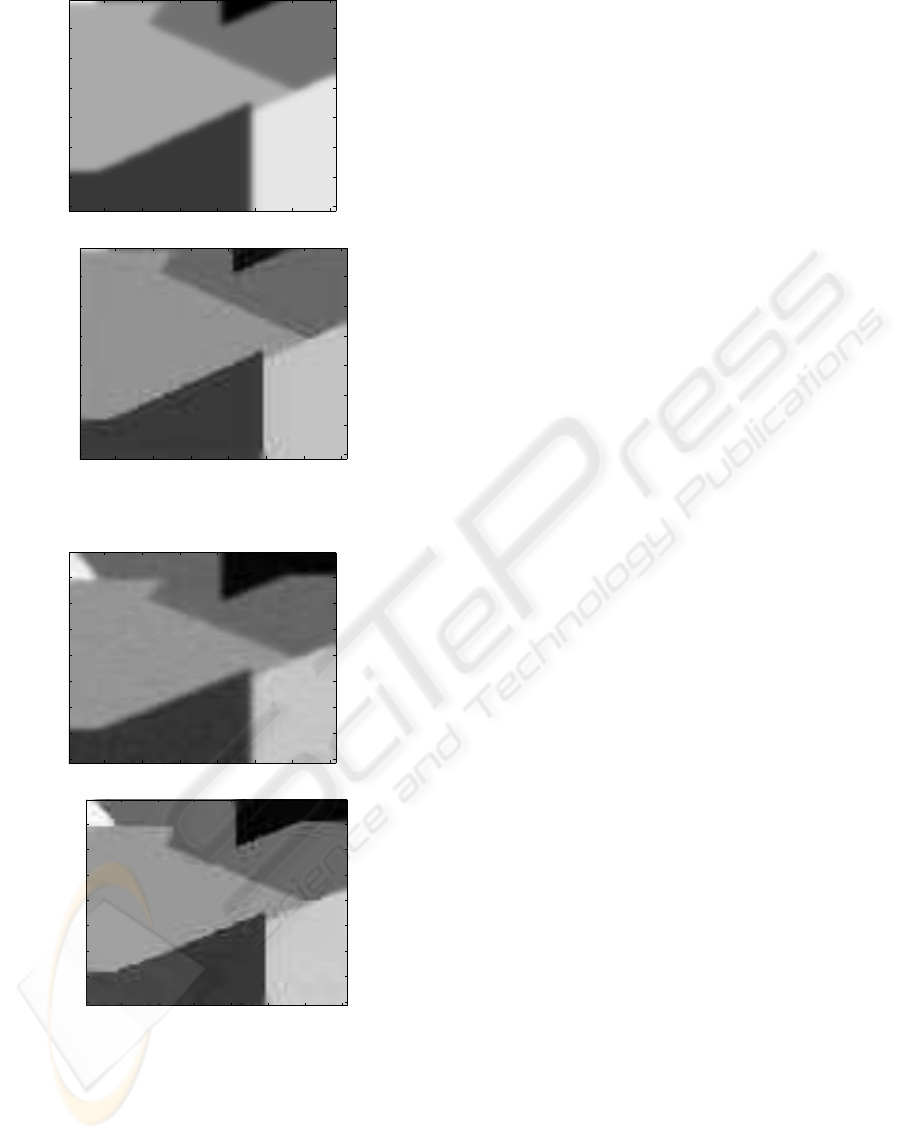
We finally obtained interesting results with this al-
gorithm. Results on the synthetic image with the same
parameters of noise and blur as for the tests in section
3.1 are shown on figure 5.
The edges are recovered well. The result is as good
as the image obtained in section 3.1 with the known
kernel.
The result image is satisfying. We have recovered
the edges without introducing artifacts. The result is
as good as the one we obtained in section 3.1 (known
kernel).
IMAGE DECONVOLUTION USING A STOCHASTIC DIFFERENTIAL EQUATION APPROACH
163
10 20 30 40 50 60 70
10
20
30
40
50
60
70
10 20 30 40 50 60 70
10
20
30
40
50
60
70
Figure 4: Blurred image top and Recovered image (bottom).
10 20 30 40 50 60 70
10
20
30
40
50
60
70
80
10 20 30 40 50 60 70
10
20
30
40
50
60
70
80
Figure 5: Blurred and noisy (σ = 3) image (top) and Result
(bottom).
4 CONCLUSION
We have shown that embedding the deconvolution
problem into a stochastic framework allows to build
solutions which avoid the local minima of the func-
tionnal, which is defined by a MRF modeling in our
case. The stochastic differential equation framework
appears to be a good alternative to the classical Gibbs
sampler approach. When the kernel is known, we
have obtained satisfactory solutions. However, faster
algorithms such as inverse filtering lead to similar re-
sults and require less computational time (Andrews
and Hunt, 1977). In the case of blind deconvolution,
we have shown that the problem is not enough con-
straint to exibit a unique solution. Therefore, some
prior on the kernel has to be considered. When using
a parametric model for the kernel, we obtained sat-
isfactory results by comnsidering a mixutre between
the proposed Langevin dynamics and the Metropolis
algorithm. This case of myopic deconvolution is the
main motivation for using the proposed approach. Fu-
ture work will consist of parameter estimation.
REFERENCES
Andrews, H. and Hunt, B. (1977). Digital image restora-
tion. Prentice Hall, Englewood Cliffs, NJ.
Descombes, X. and Zhizhina, E. (2004). Applications of
gibbs fields methods to image processing problems.
Problems of Information Transmission, 40(3):279–
295.
Geman, S. and Geman, D. (1984). Stochastic relaxation,
Gibbs distribution and the Bayeian restoration of im-
ages. IEEE Trans. on Pattern Analysis and Machine
Intelligence, 6(6):721–741.
Geman, S. and Reynolds, G. (1992). Constrained
restoration and recovery of discontinuities. IEEE
Trans. on Pattern Analysis and Machine Intelligence,
14(3):367–383.
Kloeden, P. and Platen, E. (1992). Numerical Solution of
Stochastic Differential Equations. Springer Verlag,
Berlin, Heidelberg.
Mignotte, M. (2006). A segmentation-based regularization
term for image restoration. IEEE Trans. on Image
Processing, 15(7):1973–1984.
Molina, R., Katsaggelos, A., Mateos, J., Hermoso, A., and
Segall, A. (2000). Restoration of severely blurred high
range images using stochastic and deterministic relax-
ation algorithms in compound Gauss-Markov random
fields. Pattern Recognition, 33(4):555–571.
VISAPP 2007 - International Conference on Computer Vision Theory and Applications
164
