
BAYESIAN SEPARATION OF DOCUMENT IMAGES WITH HIDDEN
MARKOV MODEL
Feng Su
†∗
, Ali Mohammad-Djafari
†
†
Laboratoire des Signaux et Systemes, UMR 8506 (CNRS-Supelec-UPS)
Supelec, Plateau de Moulon, 3 rue Joliot Curie, 91192 Gif-sur-Yvette, France
∗
State Key Laboratory for Novel Software Technology, Nanjing University, 210093 Nanjing, P. R. China
Keywords:
Blind Source Separation, document image, Bayesian estimation, HMM, MCMC.
Abstract:
In this paper we consider the problem of separating noisy instantaneous linear mixtures of document images in
the Bayesian framework. The source image is modeled hierarchically by a latent labeling process representing
the common classifications of document objects among different color channels and the intensity process of
pixels given the class labels. A Potts Markov random field is used to model regional regularity of the classi-
fication labels inside object regions. Local dependency between neighboring pixels can also be accounted by
smoothness constraint on their intensities. Within the Bayesian approach, all unknowns including the source,
the classification, the mixing coefficients and the distribution parameters of these variables are estimated from
their posterior laws. The corresponding Bayesian computations are done by MCMC sampling algorithm. Re-
sults from experiments on synthetic and real image mixtures are presented to illustrate the performance of the
proposed method.
1 INTRODUCTION
Blind source separation (BSS) is an active research
topic of signal and image processing in recent years.
It considers separating a set of unknown signals from
their observed mixtures, with reasonable assumptions
of the form of the mixing process: linear or nonlin-
ear, instantaneous or convoluting, under or over de-
termined, noisy or noiseless, and so on. However, in
all cases the mixing coefficients remain unknown and
have to be estimated as well as original source signals.
Various methods and models have been proposed
for BSS task, among which Principal Component
Analysis (PCA) seeks orthogonal directions of max-
imum variance exhibited by the data as source axes,
while Independent Component Analysis (ICA) (Hy-
varinen et al., 2001), in its basic form, assumes
statistical independency of sources and linear mix-
ing process and consists of seeking an inverse linear
transformation matrix applying on the data to achieve
maximum mutual independencybetween output com-
ponents. Both methods exploits basic statistical char-
acteristics of source signals to achieve the separation,
which makes them well generalizable and robust in
cases that as few prerequisite assumptions as uncor-
relatedness or independency can be made about the
source. Some variant algorithms are also proposed to
adapt to certain relaxation of model assumptions like
nonlinearity or noises (Harmeling, 2003; Almeida,
2005). However, in many other cases, we may find
the availability or the needs of various types of prior
information to regulate the essentially ill-posed BSS
problem. Compared with PCA and ICA, Bayesian
framework allows convenient introduction of these
prior constraints about the sources and the mixing
coefficients, and more important, supports flexible
structuring and integrating multiple hierarchical clues
for separation purpose.
In the field of image processing, BSS approaches
are being widely employed to separate or seg-
ment mixed images observed from, for example,
satelite and hyper-spectral imaging (Snoussi and
Mohammad-Djafari, 2004; Parra et al., 2000; Macias-
Macias et al., 2003), medical imaging (Calhoun and
Adali, 2006; Snoussi and Calhoun, 2005), and other
superimpositions of natural images (Bronstein et al.,
2005; Castella and Pesquet, 2004).
This paper focuses on one specific type of im-
151
Su F. and Mohammad-Djafari A. (2007).
BAYESIAN SEPARATION OF DOCUMENT IMAGES WITH HIDDEN MARKOV MODEL.
In Proceedings of the Second International Conference on Computer Vision Theory and Applications, pages 151-156
DOI: 10.5220/0002064601510156
Copyright
c
SciTePress

ages - document images, where superimposition of
two images usually appears as a major type of degra-
dation encountered in digitization (Sharma, 2001) or
ancient documents (Drira, 2006). The former degra-
dation usually occurs as artifact during scanning a
double-sided document when the text on the back-
side printing shows through the non-opaque medium
and are mixed with the foreside text. Fig.1a shows
one such example. The latter cause of text superim-
position, usually called bleed-through, can often be
observed in old documentations due to ink blurring
or penetrating as illustrated by Fig.1b. Other forms
of overlapped patterns, like underwriting and water-
marks, are also common. Though the actual under-
lying mixing process may be quite complicated and
diverse in various mixture forms, the linear mixing
model usually serves as a resonable approximation
and benefits analytical and computational simplicity,
thus is adopted in most document separation cases.
To separate document image mixtures, the com-
mon PCA and ICA algorithms can be used and have
shown their effectiveness in detecting independent
document features like watermarks, as inspected in
(Tonazzini et al., 2004) where each source was con-
sidered as random signal sequence in a whole without
further internal structuring. The Bayesian framework
has also been used before for document separation as
in (Tonazzini et al., 2006), where the source is mod-
eled by a Markov Random Field on the pixel values
to account for local smoothness inside one object, as
well as an extra line process enforcing the discontinu-
ity at object edges.
In this contribution, we propose a solution to
jointly separate and segment linearly mixed document
images. Besides considering the mixture in single
grayscale channel, we address the joint separation of
multi-channel mixture of multiple sources. In section
2, we give the probability formulation of the problem.
In section 3, the algorithm of Bayesian estimation for
model parameters is described. In section 4, simula-
tion results of the proposed algorithm are shown on
both synthetic and real images.
(a) (b)
Figure 1: Examples of mixed document images: a) show-
through mixture; b) bleed-through mixture.
2 MODEL ASSUMPTION AND
FORMULATION
Document images are created by various digitization
methods from vast types of documentation. Com-
monly, a color scanner can be used to produce three
different views of one document in the red, green,
and blue channels. With detectors working in non-
visible wavelengths such as infrared and ultraviolet,
even more information channels of data can be ob-
tained, depending on the object of interest in docu-
ments.
Given observations of M different mixtures, either
in grayscale or multiple channels, our work is thus
to obtain N corresponding source images (normally
M > N) in the same pixel format as the observations.
2.1 Data Model
In this work, the observations are M registered im-
ages (X
i
)
i=1...M
, which are defined on the same set
of pixels R : X
i
= {x
i
(r)}
r∈R
. The observations are
noisy linear instantaneous mixture of N source im-
ages (S
j
)
j=1...N
also defined on R , following the data
generation model given by:
x(r) = As(r) + n(r) r ∈ R (1)
where A = (a
ij
)
M×N
is the unknown mixing ma-
trix, n(r) is a set of independent zero-mean white
Gaussian noise for each observation with variance
σ
2
ε
= (σ
2
ε1
. . . σ
2
εM
), x(r) and s(r) are the observa-
tion and source vector at pixel r respectively. Let
S = {s(r), r ∈ R }, X = {x(r), r ∈ R }, and denote
the noise covariance matrix by R
ε
= diag[σ
2
ε1
. . . σ
2
εM
],
we have the Gaussian distribution for the observations
given the sources and the mixing parameters:
p(X|S, A, R
ε
) =
∏
r
N (As(r), R
ε
) (2)
2.2 Source Model
We model the distribution of pixel intensity for each
source images (and for each color channel) by a Mix-
ture of Gaussians (MoG), whose components cor-
respond to each object type (or class) that appears
roughly equal pixel values. For example, the simplest
model may consist of two components, one for fore-
ground text and the other for background blank. Fur-
thermore, to allow imposing constraints on distribu-
tion of class labels, for every source S
j
we represent
the class labels by a set of discrete hidden variables
Z
j
= {z
j
(r), r ∈ R } with z
j
(r) taking values from
{1, . . . , K
j
}, where K
j
is the total number of classes
VISAPP 2007 - International Conference on Computer Vision Theory and Applications
152

in image S
j
. In the following, we assume all {K
j
}
equal to the same value K.
Given pixel labels, pixels of different classes can
be reasonably assumed independent, while concern-
ing the pixels inside a given class, there are usually
two choices:
1. We may assume pixel intensities are conditionally
independent given their labels;
2. Alternatively, we may explicitly take into account
the local dependency between neighboring pixels
of same class.
In the first choice, the distribution of pixel r in the
j
th
source is modeled by:
p(s
j
(r)|z
j
(r) = k) = N (µ
jk
, σ
2
jk
) (3)
where µ
jk
and σ
2
jk
are the mean and variance of the
k
th
Gaussian component of the j
th
source. Assuming
independency between different sources and denoting
the set of labels corresponding to every source by Z =
{Z
j
, j = 1. . . N}, we have:
p(S|Z) =
∏
j
∏
k
∏
{r:z
j
(r)=k}
p(s
j
(r)|z
j
(r) = k)
which is by (3) also a Gaussian and spatially separable
on r.
In the second choice, the local dependency can be
accounted by extra smoothness constraints, like the
mean value, between neighboring pixels. We first as-
sign a binary valued contour flag q
j
(r) for every pixel
r of every source j, which is deterministicly computed
by:
q
j
(r) =
1 if z
j
(r
′
) = z
j
(r), ∀r
′
∈ V (r)
0 else
where V (r) denotes the neighbor sites of the site r.
Then, based on the value of the contour flag and
possibly current values of the neighboring pixels, the
distribution of intensity of individual pixel is formu-
lated as:
p(s
j
(r)|z
j
(r) = k, s
j
(r
′
), r
′
∈ V (r)) = N ( ¯s
j
(r),
¯
σ
2
j
(r))
(4)
with,
¯s
j
(r) = q
j
(r)µ
jk
+ (1− q
j
(r))
1
|V
jk
(r)|
∑
r
′
∈V
jk
(r)
s
j
(r
′
)
¯
σ
2
j
(r) = q
j
(r)σ
2
jk
+ (1− q
j
(r))σ
2
j
where V
jk
(r) denotes the intersection of V (r) with
the site set R
jk
= {r : z
j
(r) = k}, σ
2
j
is the a prior
variance of pixel values inside a region. Eqn.(4) states
that at the contour pixel intensities follow the Gauss
distribution whose parameters are determined by the
class labels as (3), while inside a region the distri-
bution parameters are computed from the neighbor-
ing pixels. Note that under this assumption, p(S|Z)
is no longer separable on r, but with the paral-
lel Gibbs sampling scheme proposed in (Feron and
Mohammad-Djafari, 2005), it can still be simulated
efficiently.
As a commonly observed property of visual ob-
jects, pixels belonging to the same object usually con-
nect to each other in a neighborhood of space, form-
ing several connected regions of uniformly classified
pixels, for instance, the multiple components consti-
tuting a text. By class labels defined earlier, this im-
plies regional smoothness of the spatial distribution of
class labels. This can be naturally modeled by a prior
Potts Markov Random Field for every label process
z
j
(r):
p(z
j
(r), r ∈ R ) ∝ exp
β
j
∑
r∈R
∑
r
′
∈V (r)
δ(z
j
(r) − z
j
(r
′
))
(5)
The parameter β reflects the degree of smoothing in-
teractions between pixels and controls the expected
size of the regions. In our work, all {β
j
} are as-
sumed equal and assigned an empirical value within
[1.5, 2.0].
2.3 Multiple Channels
When multi-channel image data are considered, there
are multiple options for the processing model. We can
perform separation of sources independently in each
channel and by some measures merge the results in
the end. Or, we may consider joint demixing for all
channels. In the latter case, the mixing model can still
have more alternatives:
a) all channels are equally mixed with the same mix-
ing matrix;
b) the mixing occurs separately in each channel with
different mixing matrices;
c) cross-channel mixing is assumed to be present.
In the case of a), samples from different channels of
the same observation can be concatenated for esti-
mation of the mixing coefficients, which is similar
to the monochrome case. In the case of c), an ex-
panded mixing matrix A
ML×NL
(supposing L chan-
nels) is used for all channels of all sources.
In this work, we assume the model b), where
the mixing in different channels are mutually in-
dependent and with their own separate coeffi-
cients. Thus, in RGB color format, the sources
BAYESIAN SEPARATION OF DOCUMENT IMAGES WITH HIDDEN MARKOV MODEL
153

and observations are actually {S
r
j
, S
g
j
, S
b
j
}
j=1...N
and
{X
r
i
, X
g
i
, X
b
i
}
i=1...M
. Correspondingly, there are
{A
r
, R
r
ε
, µ
r
jk
, . . . A
b
, R
b
ε
, µ
b
jk
} and so on. But for each
source S
j
, only one classification field Z
j
is main-
tained and shared by all channels, as a natural way
to enforce the common segmentation among dif-
ferent channels. This two-level hierarchical source
model, which also facilitates introducing segmenta-
tion constraints like discontinuity and local regional
dependency, is the main difference with the work of
(Tonazzini et al., 2006), where a one-level MRF mod-
eling of sources is defined on the single-channel pixel
intensities along with an explicit binary edge process.
3 BAYESIAN ESTIMATION OF
MODEL PARAMETERS
The unknown variables we want to estimate in the
models givenaboveare {S, Z, A, θ}, θ representing all
hyperparameters. The Bayesian estimation approach
consists of deriving the posterior distribution of all
the unknowns given the observation and then based
on this distribution, employing appropriate estimators
such as Maximum A Posteriori (MAP) or the Poste-
rior Means (PM) for them. With our model assump-
tions, this posterior distribution can be expressed as:
p(S, Z, θ|X) ∝ p(X|S, A, R
ε
)p(S|Z, θ
s
)p(Z)p(θ)
(6)
where, θ
s
= {(µ
jk
, σ
2
jk
), j = 1. . . N, k = 1. . . K} and
θ = {A, R
ε
, θ
s
}.
3.1 Prior Assignments for Model
Parameters
According to the linear mixing model and all
Gaussian assumptions, we choose correspondingcon-
jugate priors for model hyperparameters.
• Gaussian for source means
µ
jk
∼ N (µ
k0
, σ
2
k0
)
• Inverse Gamma for source variances
σ
2
jk
∼ I G(α
k0
, β
k0
)
• Inverse Wishart for noise covariance
R
−1
ε
∼ W
i
(α
ε
0
, β
ε
0
)
In this work, we assign uniform prior to A for sim-
plicity and no preference of the mixing coefficients,
while in other cases prior distributions like Gamma
may be used to enforce positivity.
3.2 Estimation by MCMC Sampling
Given the joint a posteriori distribution (6) of all un-
known variables, we use the Posterior Means as the
estimation for them. Since direct integration over z
is intractable, MCMC methods are employed in the
actual Bayesian computations. In our work, a Gibbs
sampling algorithm is used to generate a set of sam-
ples for every variable to be estimated, according to
its full-conditional a posteriori distribution given all
other variables fixed to their current values. Then, af-
ter certain burn-in runs, sample means from further
iterations are used as the Posterior Means estimation
for the unknowns. The algorithm takes the form:
Repeat until converge,
1. simulate S
′
∼ p(S|Z, θ, X)
2. simulate Z
′
∼ p(Z|S
′
, θ, X)
3. simulate θ
′
∼ p(θ|Z
′
, S
′
, X)
Below we give the expressions of related conditional
probability distributions.
• Sampling Z ∼ p(Z|X, S, θ) ∝ p(X|Z, θ)p(Z):
p(X|Z, θ) =
∏
r
p(x(r)|z(r), θ)
=
∏
r
N (Am
z(r)
, AΣ
z(r)
A
t
+ R
ε
)
where, m
z(r)
= [µ
1z
1
(r)
, . . . , µ
Nz
N
(r)
]
t
and Σ
z(r)
=
diag[σ
2
1z
1
(r)
, . . . , σ
2
Nz
N
(r)
].
Notice p(Z) =
∏
N
j=1
p(z
j
), and as mentioned ear-
lier, p(z
j
) takes the form of Potts MRF as (5).
An inner Gibbs sampling is then used to simulate
z
j
with the likelihood p(x(r)|z(r), A, θ) marginal-
ized over all configurations of {z
j
′
(r), j
′
6= j}.
• Sampling S ∼ p(S|X, Z, θ):
p(S|X, Z, θ) ∝ p(X|S, A, R
ε
)p(S|Z, θ)
=
∏
r
N (m
apost
s
(r), R
apost
s
(r))
R
apost
s
(r) =
h
A
t
R
−1
ε
A+ Σ
−1
z(r)
i
−1
m
apost
s
(r) = R
apost
s
(r)
h
A
t
R
−1
ε
x(r) + Σ
−1
z(r)
m
z(r)
i
• Sampling R
ε
:
p(R
ε
|X, S, A) ∝ p(X|S, A, R
ε
)p(R
ε
)
Considering we assign an inverse Wishart distri-
bution to p(R
ε
), which is conjugate prior for the
likelihood (2), R
ε
is a posteriori sampled from:
R
−1
ε
∼ W
i
(α
ε
, β
ε
)
α
ε
=
1
2
(|R |− n), β
ε
=
1
2
|R |(R
xx
− R
xs
R
−1
ss
R
t
xs
)
where, the sample statistics R
xx
=
1
|R |
∑
r
x
r
x
t
r
,
R
xs
=
1
|R |
∑
r
x
r
s
t
r
, R
ss
=
1
|R |
∑
r
s
r
s
t
r
.
VISAPP 2007 - International Conference on Computer Vision Theory and Applications
154
• Sampling A ∼ p(A|X, S, R
ε
):
p(A|X, S, R
ε
) ∝ p(X|S, A, R
ε
)p(A)
Given uniform or Gaussian prior for A, the poste-
rior distribution of A is a Gaussian:
Vec(A) ∼ N (µ
A
, R
A
)
µ
A
= Vec(R
xs
R
−1
ss
), R
A
=
1
|R |
R
−1
ss
⊗ R
ε
where ⊗ is the Kronecker product and Vec(.) rep-
resents the column-stacking operation.
• Sampling (µ
jk
, σ
2
jk
):
With (Z, S) sampled in earlier steps and conjugate
priors assigned, the means µ
jk
and the variances
σ
2
jk
can be sampled from respective posteriors as
follows:
µ
jk
|s
j
, z
j
, σ
2
jk
∼ N (m
jk
, v
2
jk
)
m
jk
= v
2
jk
µ
k0
σ
2
k0
+
1
σ
2
jk
∑
r∈R
( j)
k
s
j
(r)
v
2
jk
=
n
( j)
k
σ
2
jk
+
1
σ
2
k0
−1
and,
σ
2
jk
|s
j
, z
j
, µ
jk
∼ I G(α
jk
, β
jk
)
α
jk
= α
k0
+
n
( j)
k
2
β
jk
= β
k0
+
1
2
∑
r∈R
( j)
k
(s
j
(r) − µ
jk
)
2
where, label region R
( j)
k
= {r : z
j
(r) = k} and the
region size n
( j)
k
= |R
( j)
k
|.
4 SIMULATION RESULTS
For evaluating the performance of the proposed algo-
rithm, we use both synthetic and real images in the
test. The synthetic images were generated according
to the model setting that each source is composed of
pixels of two classes (text and background) and two
source images are linearly mixed in every color chan-
nel independently to produce two observation images.
This was done in three steps:
1. Two binary (K
j=1,2
= 2) text image were scanned
from real documents or created by graphic tools.
They were used as the class labels Z
j=1,2
for each
source;
2. With known means and variances for pixel value
of each class, the source images were generated
according to (3);
3. For each color channel, a random selected A
2×2
was used to mix the sources and finally white
Gaussian noises R
ε
were added (SNR=20dB).
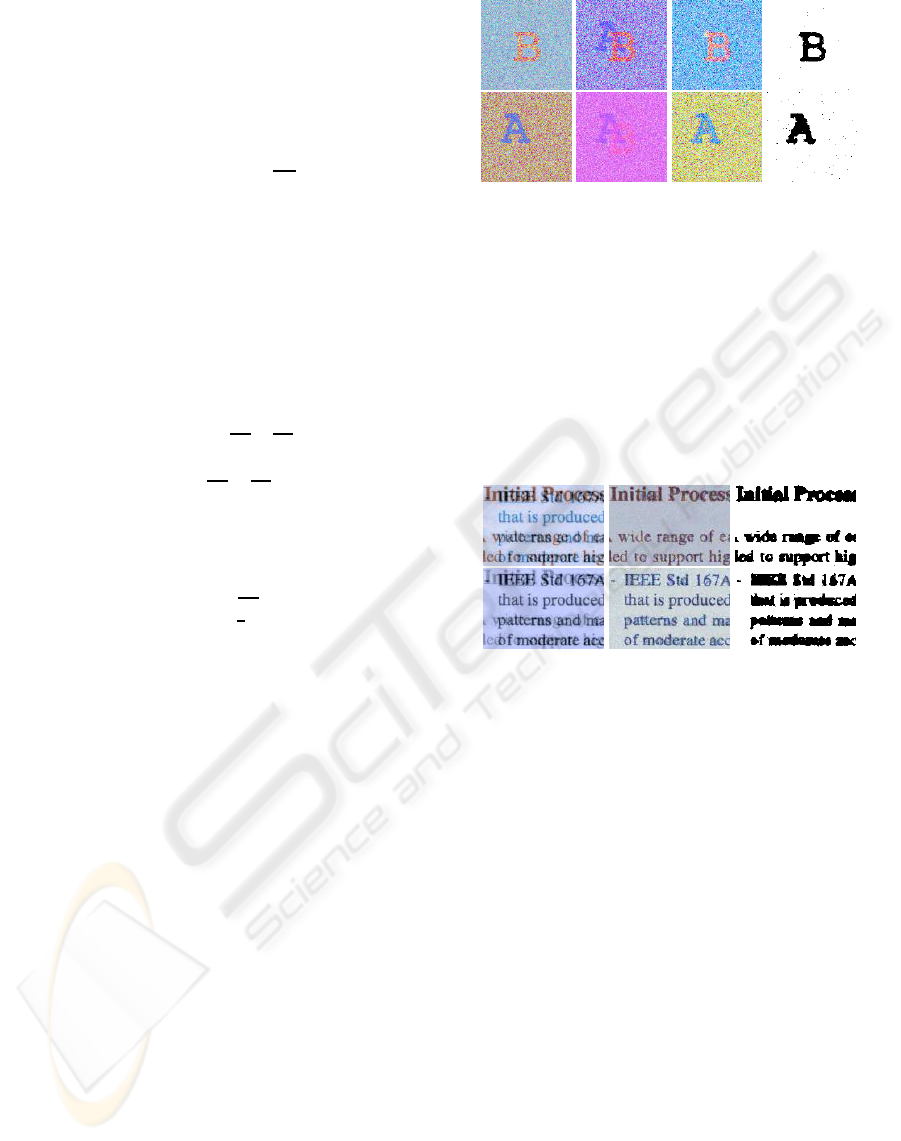
(a) (b) (c) (d)
Figure 2: Separation of synthetic image mixtures: a) origi-
nal sources; b) image mixtures; c) demixed sources; d) clas-
sification labels.
Fig.2 shows the synthetic image mixtures, demixed
sources and the label fields.
The real image for test was scanned from a duplex
printed paper, where show-through causes the super-
imposition of text. The separation result is shown in
Fig.3.
(a) (b) (c)
Figure 3: Separation of real show-through image mixtures:
a) image mixtures; b) demixed sources; c) classification la-
bels.
For comparison, we also employed the FastICA
algorithm (Hyvarinen, 1999) on the sample images
with typical parameter set. The results on the show-
through examples of Fig.3 are shown in Fig.4. All
three channels of the two observed mixtures were
used as inputs simultaneously to the ICA algorithm.
The two demixed sources can be found in two of
six independent components (IC) outputed, while
the other four output ICs usually contain unintended
noise-like signals, which, along with the permutabil-
ity property of the ICA algorithm, bring difficulties
to reconstructing color representation of the sources.
On the other hand, when less color channels are ex-
ploited in demixing, we noticed that the separation
result does not necessarily degrade or improve, owing
to the possible presence of cross-channel correlations.
The MCMC computation involvedin the proposed
Bayesian separation method is time-consuming. For
the example image of 300x240 pixels in Fig.3, which
is small relative to ordinary document sizes and res-
olutions, the typical computation time of the experi-
BAYESIAN SEPARATION OF DOCUMENT IMAGES WITH HIDDEN MARKOV MODEL
155

(a) two ICs corresponding to the demixed sources
(b) other ICs containing noise-like signals
Figure 4: Separation results by ICA.
mental implementation can come up to hours without
specific optimizations. However, various computing
alternatives such as Mean Field and variational ap-
proximation can be exploited to achieve higher effi-
ciency.
5 CONCLUSION
We proposed a Bayesian approach for separating
noisy linear mixture of document images. For source
images, we considered a hierarchical model with
the hidden label variable z representing the common
classification of objects among multiple color chan-
nels, and a Potts-Markov prior was employed for the
class labels imposing local regularity constraints. We
showed how Bayesian estimation of all unknowns of
interest can be computed by MCMC sampling from
their posterior distributions given the observation. We
then illustrated the feasibility of the proposed algo-
rithm on joint separation and segmentation by tests
on sample images.
REFERENCES
Almeida, L. B. (2005). Separating a real-life nonlinear im-
age mixture. Journal of Machine Learning Research,
6:1199–1232.
Bronstein, A. M., Bronstein, M. M., Zibulevsky, M., and
Zeevi, Y. Y. (2005). Sparse ICA for blind separation
of transmitted and reflected images. Intl. Journal of
Imaging Science and Technology (IJIST), 15:84–91.
Calhoun, V. D. and Adali, T. (2006). Unmixing fMRI with
independent component analysis. IEEE Engineering
in Medicine and Biology Magazine, 25(2):79–90.
Castella, M. and Pesquet, J.-C. (2004). An iterative blind
source separation method for convolutive mixtures
of images. Lecture Notes in Computer Science,
3195/2004:922–929.
Drira, F. (2006). Towards restoring historic documents
degraded over time. In Second International Con-
ference on Document Image Analysis for Libraries,
pages 350–357.
Feron, O. and Mohammad-Djafari, A. (2005). Image fusion
and unsupervised joint segmentation using HMM and
MCMC algorithms. Journal of Electronic Imaging,
14(2).
Harmeling, S. (2003). Kernel-based nonlinear blind source
separation. Neural Computation, 15(5):1089–1124.
Hyvarinen, A. (1999). Fast and robust fixed-point algo-
rithms for independent component analysis. IEEE
Transactions on Neural Networks, 10(3):626–634.
Hyvarinen, A., Karhunen, J., and Oja, E. (2001). Indepen-
dent Component Analysis. John Wiley & Sons, Inc.,
New York.
Macias-Macias, M., Garcia-Orellana, C. J., Gonzalez-
Velasco, H., and Gallardo-Caballero, R. (2003). In-
dependent component analysis for cloud screening of
meteosat images. In International Work-conference
on Artificial and Natural Neural Networks (LNCS
2687/2003), volume 2687, pages 551–558.
Parra, L., Spence, C., Ziehe, A., Muller, K.-R., and Sajda, P.
(2000). Unmixing hyperspectral data. In Advances in
Neural Information Processing Systems, volume 12,
pages 942–948.
Sharma, G. (2001). Show-through cancellation in scans of
duplex printed documents. IEEE Transactions on Im-
age Processing, 10(5):736–754.
Snoussi, H. and Calhoun, V. D. (2005). Bayesian blind
source separation for brain imaging. In IEEE Interna-
tional Conference on Image Processing (ICIP) 2005,
volume 3, pages 581–584.
Snoussi, H. and Mohammad-Djafari, A. (2004). Fast joint
separation and segmentation of mixed images. Jour-
nal of Electronic Imaging, 13:349–361.
Tonazzini, A., Bedini, L., and Salerno, E. (2006). A markov
model for blind image separation by a mean-field EM
algorithm. IEEE Transactions on Image Processing,
15(2):473–482.
Tonazzini, A., Salerno, E., Mochi, M., and Bedini, L.
(2004). Blind source separation techniques for de-
tecting hidden texts and textures in document images.
In ICIAR 2004, LNCS 3212, pages 241–248, Berlin.
Springer-Verlag.
VISAPP 2007 - International Conference on Computer Vision Theory and Applications
156
