
CIRCULAR PROCESSING OF THE HUE VARIABLE
A Particular Trait of Colour Image Processing
Alfredo Restrepo Palacios, Carlos Rodríguez and Camilo Vejarano
Laboratorio de Señales, Dpt. Ing. Eléctrica y Electrónica
Universidad de los Andes, Bogotá, Colombia
Keywords: Colour image processing, angular data, hue, median filter, range filter, von Mises distribution, mathematical
morphology.
Abstract: Novel tools for colour image processing are presented. Unlike many magnitudes dealt with in engineering,
the hue variable of a colour image is circular and requires a special treatment. Special techniques have been
advanced in statistics for the analysis of data from angular variables; likewise in image processing for the
processing of the hue variable. We give a definition of the median and of the range of angular data and
apply their running versions on images to smooth them and to detect hue edges. We also give definitions of
hue morphology; one based on the topological concept of lifting and on grey level morphology; another
definition is wholly given in a circular context.
1 INTRODUCTION
We consider a specific aspect of colour image
processing, namely the processing of the H variable
of the HVS colour system. The H variable is an
angular variable, i.e. one that lives in the circle
which is the one dimensional sphere S
1
, that we
interpret as the one-point compactification of the
interval (–π, π]. S
1
is orientable; we assume that the
orientation is positive when it is counterclockwise;
in this sense, colours are positively sequenced as in
red, orange, yellow, citrine, green, cyan, blue violet,
red etc.; see Figure 1. Unless otherwise stated, in the
examples, we assume V = S = 0.8 (constant value
and saturation). The tools given here can be
combined with other tools that process the V and S
variables.
The elements of S
1
cannot be linearly ordered in
any way compatible with its topology; thus, a
circular version of most statistics already defined for
linearly ordered data is usually not obvious. A
typical problem for the definition of location
statistics is that for certain uniformly distributed
samples it is best to leave them undefined; e.g. the
average of a sample of equally spaced angles. Also,
the problem of multiplicity is more ubiquitous than
in the case of a linearly ordered range space (e.g., in
the linearly ordered case, the median of an even
sized sample). We consider four sample statistics:
the circular average, a circular median, a circular
range and the circular concentration, and their
corresponding running versions.
Red=0
Yellow=0.5š
Green=š
Blue=-0.5š
Figure 1: The space S
1
of hues.
A 2D image (i.e. a 2D signal) h:A→B is a
function whose domain set A is two dimensional;
the image is discrete if A is countable, it is digital if
its range set B is finite. In the case of discrete
images, we use as domain set a product of integer
intervals. An integer interval /n, m/ is the set of the
integers less than or equal to m and larger than or
equal to n. We concentrate here on images whose
range set is S
1
; we call them hue images and picture
them as computer images in the HSV colour system
with S and V constant. The elements of the domain
set are called pixels and the elements of the range set
are the possible values of the pixels.
Several proposals for doing hue mathematical
morphology have been advanced e.g. (Peters II,
69
Restrepo Palacios A., Rodríguez C. and Vejarano C. (2007).
CIRCULAR PROCESSING OF THE HUE VARIABLE - A Particular Trait of Colour Image Processing.
In Proceedings of the Second International Conference on Computer Vision Theory and Applications - IFP/IA, pages 69-76
Copyright
c
SciTePress
Original
10 20 30 40 50
10
20
30
40
50
Circular Mean
10 20 30 40
5
10
15
20
25
30
35
40
45
Original
50 100 150 200
50
100
150
200
Mean
50 100 150
20
40
60
80
100
120
140
160
180
1997), (Comer and Delp, 1999), (Hanbury and Serra,
2001), (Hanbury and Serra, 2001), (Vejarano, 2002)
and others. We give one based on the uniqueness of
the lifting of a map (a map is a continuous function)
with domain a simply connected space to the
universal cover of the range space (Christenson and
Voxman, 1998); another, based on intrinsic aspects
of the circular relation of angular data.
2 STATISTICS OF LOCATION
AND DISPERSION FOR
DIRECTIONAL DATA
Most of the time we assume angles (i.e. hues) to be
either numbers in the interval (-π, π] or numbers in
the interval [0, 2π); the choice by default is (–π, π].
Except in the case of liftings, we do not use multiple
code representations (equivalent mod-2π) for the
same angle.
It is convenient to use the complex number e
jφ
as
a representation the angle
φ. Assuming the function
arctan to have range (-π/2, π/2); the angle arg(z) of a
nonzero complex number (arg(z) is not defined if z =
0+j0) is defined as:
arg(z)= arctan(Im(z)/Re(z)) if Re(z)>0
arg(z)= –π + arctan(Im(z)/Re(z)) if Re(z)<0
arg(z)= π/2 if Re(z)=0 and Im(z)>0
arg(z)= –π/2 if Re(z)=0 and Im(z)<0
Let [
φ
1
, … φ
N
] be a sample of N angles; unlike a
set, in a sample there may be repeated data. Let [z
1
,
… z
N
], with φ
i
=arg(z
i
), be the N-tuple of the
corresponding complex numbers on the unit circle.
We respectively call
Z :=
z
i
i=1
N
∑
and Φ = (
φ
i
i=1
N
∑
) mod-2π
the complex sum and the angular sum of the angles.
Clearly, arg(Z) ≠ Φ. For example, consider 3π/4 and
5π/4.
2.1 Sample Mean or Average
We give the standard definition of the average of a
sample of angles; see e.g. (Nicolaidis and Pitas,
1998) and (www.higp.hawaii.edu, 2006).
Let [
φ
1
, … φ
N
] be a sample of N angles; if their
complex sum Z is 0+j0, we leave the average of the
sample undefined, otherwise, the average of the
sample is set to be the angle arg(Z) of the complex
sum.
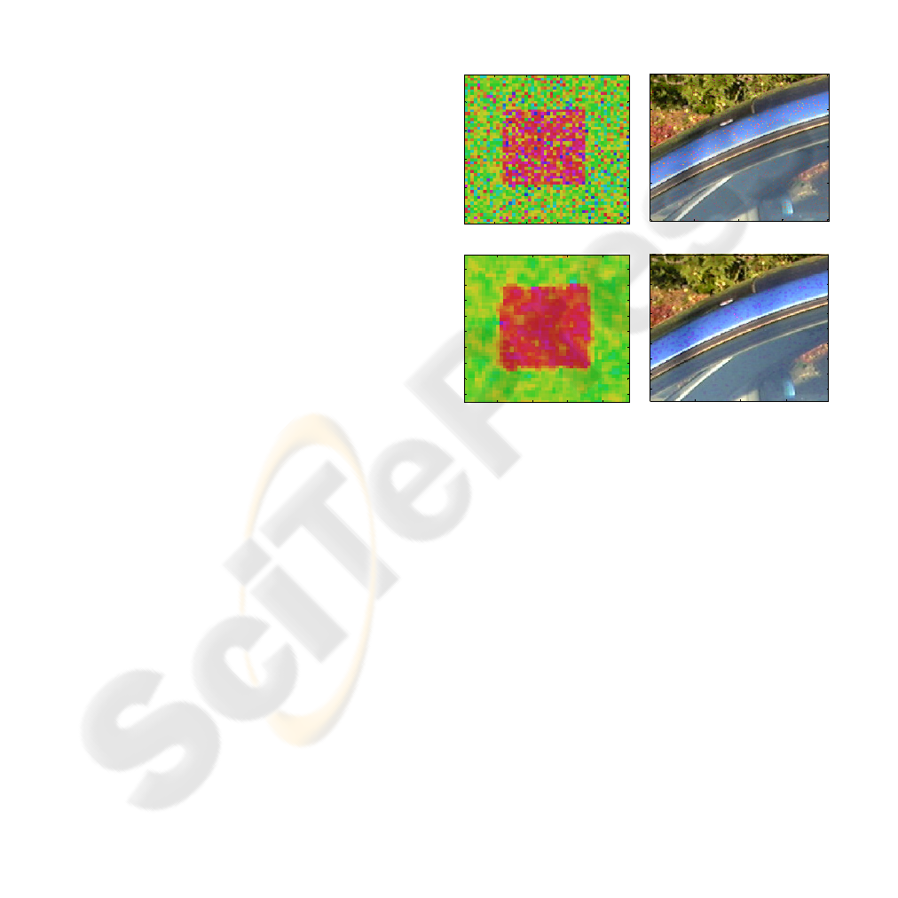
For the texture images at the top in Figure 2,
after the application of the running average (we use
windows of size 3x3) the images at the bottom
result. When the average of a window is undefined,
the central pixel was left unchanged. The textures
are based on the Von Mises distribution, given by:
f(φ) = (1/2πI
0
(κ)) exp(κ cos(φ–α))
where I
0
is a Bessel function that ensures that the pdf
integrates to 1, the parameter κ has to do with the
variance and α is the mean of the distribution.
Figure 2: A Von Mises’ texture images and a noisy image
(top) and the result after applying a moving average
(below).
2.2 Sample Median
As above, let [φ
1
, … φ
N
] be a sample of angular
data. Let d
ij
be the distances between pairs (a pair is
a set of cardinality two) of consecutive angles φ
i
and
φ
j
, given by d
ij
= T(|φ
i
– φ
j
|), where:
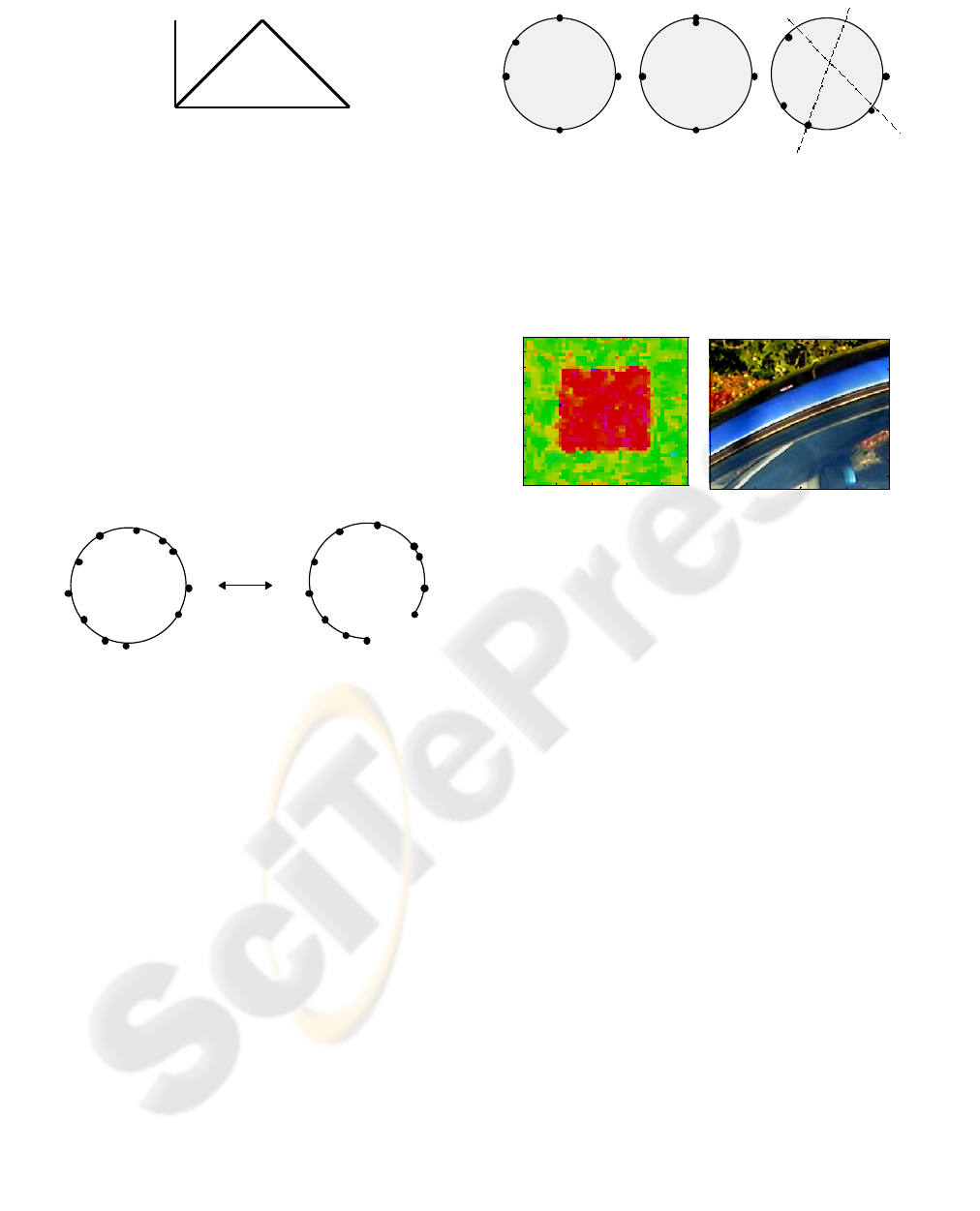
T: [0, 2π) → [0, π]
has the graph indicated in Figure 3.
To find out which angles are consecutive, order the
angles in the sample, in their domain of
representation (-π, π], get the pairs of consecutive
angles in this ordering, and add an extra pair given
by the largest and the smallest angles in this interval.
VISAPP 2007 - International Conference on Computer Vision Theory and Applications
70
Circular Median
10 20 30 40
5
10
15
20
25
30
35
40
45
Median
50 100 150
20
40
60
80
100
120
140
160
180
T(x)
π
x
0 π 2π
Figure 3: The function T, used to define a metric on S
1
.
If each component of the sample has the same
value, let the median be this common value. If the
sample is not constant, the set of distances {d
ij
} has
a positive (i.e. larger than zero) maximum; if this
positive maximum is achieved for a unique pair of
angles
φ
i
and φ
j
, subtract the 0-sphere {φ
i
, φ
j
} from
the 1-sphere S
1
; two connected components result
(Jordan theorem in dimension 1;) of these two
components, one contains the data; subtract the other
connected component, which we call the gap; the
resulting arc contains the data and and may now be
linearly ordered (see Figure 4); take the median of
the data in this arc, if the sample has even size, take
the (angular) average of the two central data.
Figure 4: The data determine a gap on S
1
, which is taken
off.
If the maximum of the distances between
consecutive angles is achieved more than once, the
definitions must be refined; see Figs. 5a. and 5b. For
one thing, the sample has several gaps of unique
length and it still may have a median. Proceed in two
steps to find it. Initially, for each of the multiple,
equally maximally sized gaps, obtain a median as
above. The resulting set of medians may further
have a median or it may not; it does not if this set of
preliminary medians determines again a unique
distance between consecutive points; in such a case
the sample is said to be uniformly spaced and to
have no median (nor a mean.) Otherwise, compute
the median of this set of preliminary medians, as
above, and call it the median of the sample.
A rule of thumb to check things is to slightly
separate repeated data. The definition given of the
sample median of angular data gives a unique
answer in cases when the median defined in
(Nicolaidis and Pitas, 1998) does not; see Figure 5c.
-a- -b- -c-
Figure 5: In a, there are three maximal gaps; in b, four. In
each case, they are of the same length.
In Figure 6, we show the result of applying a 3x3
hue median filter to the texture images at the top of
Figure 2.
Figure 6: The result of applying the median filter to the
images at the top in Figure 2.
2.3 Max and Min
Both the average and the median of a sample of hues
are hues and so are the max and the min as defined
below; nevertheless, the length of the gap, the
concentration and the range are angles but no hues:
they are differences of hues. Two different pairs of
hues may have the same difference and a sample
may have a range but no median.
Let [
φ
1
, … φ
N
] be a sample of angular data. If
the sample is uniformly spaced or if there are a
multiple gaps, the max and the minimum of the
sample are left undefined; otherwise, for a unique
gap, the maximum (max) and minimum (min) of the
sample are defined as follows: take the gap off as
above and, in the remaining arc, let the point most
ccw (counterclockwise) be the maximum of the
sample and the point most cw (clockwise) be the
minimum. For example, for the sample [orange, red,
yellow], red is the min and yellow is the max.
2.4 Concentration and Range
Let [φ
1
, … φ
N
] be a sample of angular data; let the
concentration C of the sample be given by the
magnitude of the complex sum Z divided by N,
C: = (1/N)|Z|
CIRCULAR PROCESSING OF THE HUE VARIABLE - A Particular Trait of Colour Image Processing
71
Original
200 400 600 800 1000 1200 1400 1600
200
400
600
800
1000
1200
Range
200 400 600 800 1000 1200 1400
200
400
600
800
1000
1-T(Gap)
200 400 600 800 1000 1200 1400
200
400
600
800
1000
Concentration
200 400 600 800 1000 1200 1400
200
400
600
800
1000
C ranges between 0 and 1, and clearly is a measure
of the concentration of the data. If the complex sum
of the sample is 0, the sample has no average but it
has (zero) concentration. The name given here to
this statistic is not standard (mean resultant length,
in (www.higp.hawaii.edu, 2006)).
For a constant sample, the range is set to be 2π;
otherwise, proceed as in Section 2.2 and define the
range ρ of the sample as:
ρ = 2π – max{d
ij
} = 2π – length(gap)
ρ clearly is a measure of the dispersion of the data.
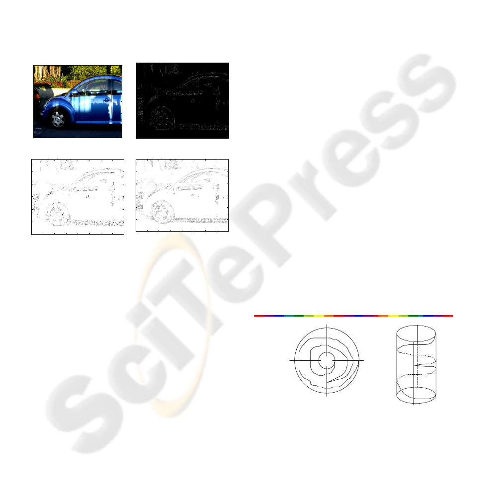
The moving range and moving concentration are
used to get maps of hue edges, from the image at the
top, left, in Figure 7.
Figure 7: Hue edge maps.
3 HUE IMAGES
A continuous 2D image (as opposed to a discrete
image as defined in Section I) is a function with
domain set a product I
×J of real intervals The
continuity referred to here is of the domain; thus, a
continuous image may be a discontinuous function.
If the range set is S
1
, the values of the function are
hues.
The existence of certain mathematical tools for
handling continuous functions makes the
corresponding images important from a theoretical
viewpoint. For example, the lifting of a continuous
function to a simply connected cover of the range
set, is unique. Thus, even though the discontinuities
of a function carry important information, it may be
convenient to restrict attention to continuous, and
even differentiable, functions. After all, the rates of
change can be arbitrarily large. In fact, the largest
possible jump of a hue image has value π and it
corresponds to a change from a hue to its opposing
hue, which may correspond as well to its
complementary colour. (Two colours are said to be
complementary if their additive mixture produces an
achromatic colour).
But, perhaps more to the point, in digital image
processing, one considers discrete images.
Moreover, in practice, discrete images are digital (as
defined in Section I); nevertheless, we disregard
here the discrete nature of the range set. The range
set of the hue component of an image, in all cases
will be assumed to be S
1
.
Since the basic definitions of mathematical
morphology are given in terms of the operations of
taking the maxima and minima of sets, it is assumed
that the range set has at least the structure of a
linearly ordered set (and the domain set, that of a
lattice). This is the case of grey level images, for
example, but not the case of hue images. We explore
below two approaches for performing morphology
on angle-valued functions; one is based on the
topological concept of the lift of a function while the
other works in the natural ambient space of the
graph of the function; both are based on grey level
morphology. Initially, we consider briefly the
geometry of the ambient space of the graph of the
hue function.
3.1 The Graph of a Function from a 2D
Interval to the Circle
Consider 1D continuous hue images. The graph of a
function f:I
→S
1
lives on I×S
1
which is a cylinder
and can be also thought of an annulus (the annulus is
homeomorphic but not isometric); if the function is
continuous, the graph is connected. See Figure 8.
RedGreen
Blue
Yellow
RedGreen
Yellow
Blue
Figure 8: Two pictures of the graph of the function
f:I→S
1
, corresponding to the coloured line, shown
discontinuous above.
The graph of a function f : I×J →S
1
lives on
I
×J×S
1
which can be thought of a solid cylinder; if
the function is continuous, the graph is connected.
VISAPP 2007 - International Conference on Computer Vision Theory and Applications
72
I
J
Figure 9: The product I
2
×S
1
.
For each s ∈ S
1
the intersection K
s
of the graph of
f with the plane {(x, s) : xI
×J} I×J×S
1
has as
connected components points, arcs, Jordan curves
and unions of these. We may give a partial order to
the set of the simple closed curves in
T
s
:= K
s
∗ ∂(I×J)
= {(x, s) : xI
×J, f(x) = s} ∗ ∂(I×J)
A simple closed curve C
1
bounds a region on its
interior (i.e. the region farthest from ∂(I
×J)); if
another Jordan curve C
2
in T
s
lies in this region, we
write C
2
< C
1
. This is a partial order.
3.2 Lifting Angular Maps
R
1
is the universal covering space of S
1
(Christenson
and Voxman, 1998), as projection map we have
p(x):= [x]
2π
where [x]
2π
is the only number in [0, 2π)
equivalent to x, mod-2π. See Figure 10.
R
1
F p
I
×J f S
1
Figure 10: R
1
is the universal cover of S
1
.
Now to lift a continuous function f:I×J→S
1
is to
find a continuous function F:I
×J→R
1
such that
p(F(x)) = f(x). If we specify F(0, 0) = f(0, 0), F is
unique.
The max minus the min of the values taken by a
lift F of a hue function f is said to be the degree of f.
It is rare that in an image of a common scene, the
degree of the hue be larger than 2π; it implies more
than one set of colours as in a rainbow, with the
same ordering of colours along some path.
To lift f is, in a sense, to unfold its graph. The
smallest curves in T
0
, according to the partial
ordering defined in Section 3.1, are the starting point
for an algorithm that finds the lift F. Find these
smallest simple closed curves and then define F on
the regions bounded by these components. Initially,
on these smallest regions set F:=f. Then, depending
on whether F is positive or negative on a region, for
the next region, define F as f+2π or f-2π. On a
region of order n, add or subtract 2nπ.
4 MATHEMATICAL
MORPHOLOGY FOR A
CONTINUOUS ANGULAR
VALUED FUNCTION
The (unique) lifting F:I×J→R
1
of a hue map
f:I
×J→S
1
, has as range set R
1
, which is linearly
ordered. We define MOP(f) as p(mop(F)); where
mop is a standard grey level morphological operator
(Heijmans, 1994), (Serra, 1998) and MOP is the
corresponding hue, morphological operator being
defined.
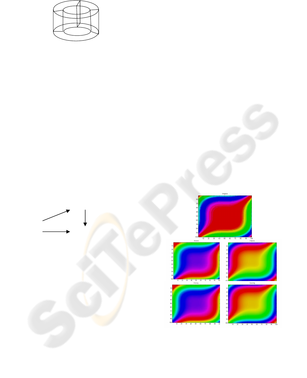
For example, the hue image in Figure 11
corresponds to the function with graph (plotted in a
flat 3D ambient space) as shown in Figure 12; the
lifting of this function is also shown in Figure 12;
applying (“grey level”) dilation/erosion and
opening/closing, with the structuring element in
Figure 13, and projecting back on S
1
with the
projection p = (mod 2π), we get the image shown in
Figure 11.
Figure 11: Hue morphology based on lifting.
As we see, for the given structuring element, in
the erosion, reds become violet, in general there is a
cw shift of hues which, for the given image, gives an
impression of migration of hues in the (opposite)
ccw direction (violets migrating toward red regions.)
CIRCULAR PROCESSING OF THE HUE VARIABLE - A Particular Trait of Colour Image Processing
73
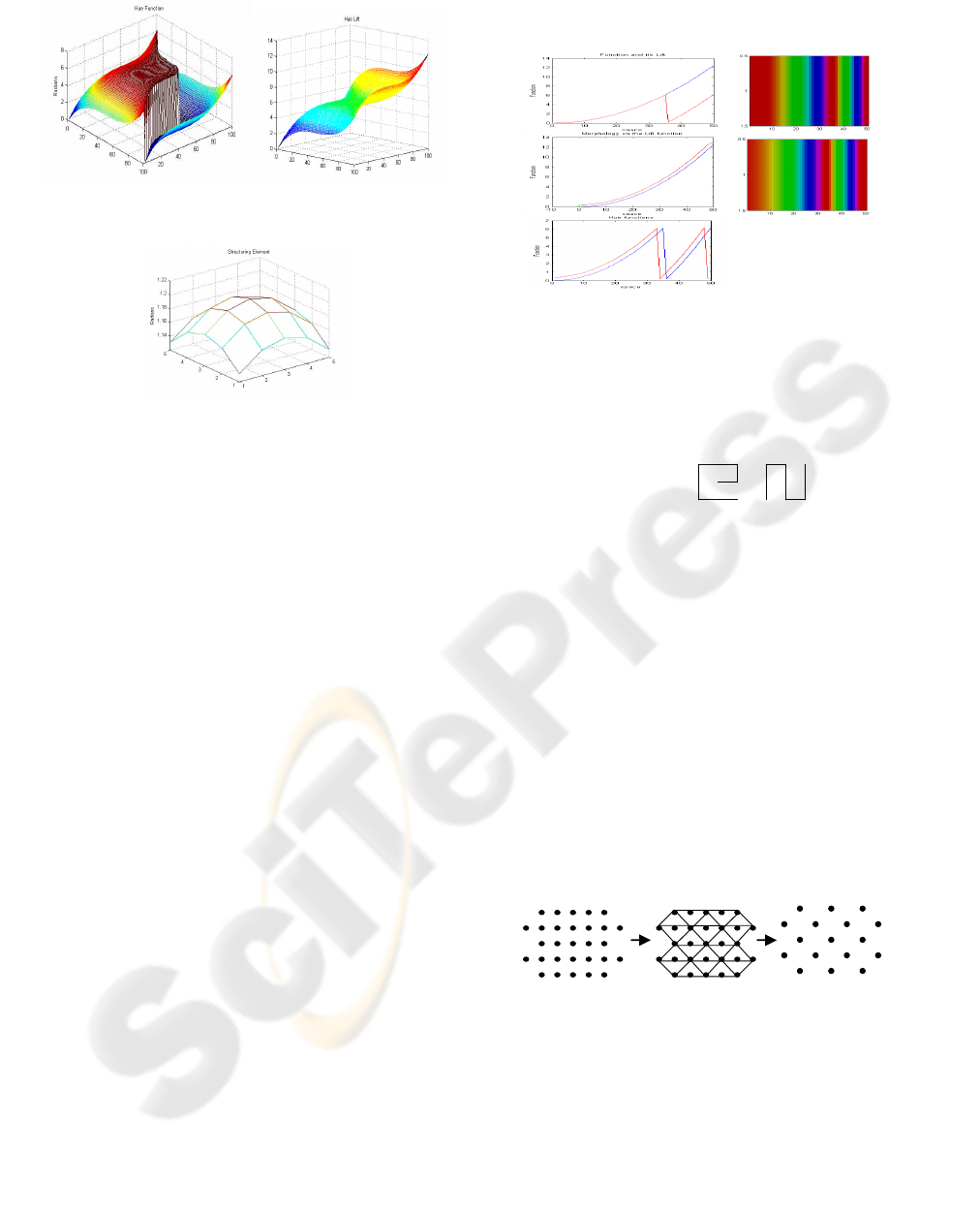
Figure 12: Hue function and lifted version (false colours).
Figure 13: Structuring element.
4.1 Algorithms for Lifting Discrete
Images
For a function f:N×M→S
1
, where N and M are
discrete intervals, several algorithms can be
proposed to obtain functions F:N
×M→R
1
such that
p(F(x)) = f(x); however, the difference between two
such F´s (we chose to call them “lifts”) is not
necessarily constant. One kind of algorithm is based
on the idea of sweeping the domain set N
×M
another kind is based on the idea of interpolating the
discrete image and obtain a continuous image.
4.1.1 Lifting Along Paths
Consider initially a coloured line, that is, a function
with domain set an integer interval /0, N-1/. We start
at either one of the extrema of the interval, say at 0.
Initially, we set F(0) = f(0), to compute the
remaining values of F, we proceed as follows.
Assume F has been defined up to pixel i; next, let
F
i+1
= F
i
+ Δ(δ
i
) where δ
i
:= f
i+1
- f
i
and Δ is
defined as Δ(δ) = δ, if |δ| < π; Δ(δ) = 2π + δ, if δ < –
π; and Δ(δ) = δ – 2π if δ > π. Clearly, f = F (mod-
2π). The algorithm does not give a unique lift. The
lift obtained starting from the right may be different.
Nevertheless, the two lifts are equivalent, i. e. their
difference is a constant congruent with 0 (mod-2π).
Then, the operators of grey-level morphology can be
applied, before projecting back on S1, See Figure
14. Now consider 2D, discrete, hue images f: /1, N/
x /1, M/
→ S
1
; a lift F of f is such that F(i, j) = f(i, j)
mod-2π. Sweeping the domain set along a simple
path gives Δs between neighbours that depend on the
path chosen to do the lift.
Figure 14: A 1D hue function and its lift, a structuring
element and the resulting function, the original function
and the projected processed function. The original 1D
image and the resulting one on the right.
For example, consider the image and the two
sweeping paths below
0 1.5π π
0.5π 0 0.5π
π 1.5π 0
the corresponding resulting lifts are
2π 1.5π 1π 0 -0.5π π
2.5π 0 0.5π 0.5π 0 0.5π
3π 3.5π 4π π -0.5π 0
4.1.2 Interpolating Hue Images
The (e.g. linear) interpolation of a function defined
on a rectangular grid ZxZ to a function defined on
ZxZ is not uniquely defined; consider 4 neighbour
pixels as in the corners of the square, notice that
there are several, possibly conflicting, ways of
interpolating along the diagonals. From an image
with a very good resolution, that won’t loose much
from a process of decimation as it is redefined on a
(non regular) hexagonal grid, discard the pixels (i, j)
for which i+j is odd, as shown in Figure 15.
Figure 15: The decimation of a rectangular grid that give a
hexagonal grid.
On each triangle linear interpolation is used.
Once again, there are multiple possible linear
interpolations, some of them of the same cost. By
cost we mean the spent arc length on the circle.
Consider first interpolation along a line. Here there
are only two possible options: for x and y are angles
in [0, 2π), assuming x≤y, there are two choices:
VISAPP 2007 - International Conference on Computer Vision Theory and Applications
74
Original
100 200 300 400
100
200
300
400
500
600
0
2
4
6
0
2
4
6
0.54
0.56
0.58
0.6
0.62
0.64
Spatial Domain
Estructuring Element function
Radians
Dilation
100 200 300 400
100
200
300
400
500
600
Opening
100 200 300 400
100
200
300
400
500
600
Clos ing
100 200 300 400
100
200
300
400
500
600
Erosion
100 200 300 400
100
200
300
400
500
600
(1-α)x+αy and [(1-α)(x+2π)+αy]
2π
; if |x-y| = T(|x-y|)
then the first choice is less expensive and if |x-y| >
T(|x-y|) then the second choice is less expensive.
The parameter α varies between 0 and 1.
Let x, y and z be three pixels which are the vertices
of a triangle and let u=f(x), v=f(y) and w=f(z) be the
corresponding hues and assume that, as numbers in
[0, 2π), u≤v≤w. There are three possible linear
interpolations for the colours of the points in the
triangle; for each point in the triangle let λ
1
, λ
2
, λ
3
be
the (unique) barycentric coordinates of the point; the
interpolations are given by [λ
1
(u+2π)+λ
2
v+λ
3
w]
2π
,
[λ
1
u+λ
2
v+λ
3
w]
2π
and [λ
1
u+λ
2
v+λ
3
(w–2π)]
2π
. The
choice depends on the cost of each interpolation and
on the choices made for neighbour triangles.
Once a continuous function is obtained, the
image has a unique lift.
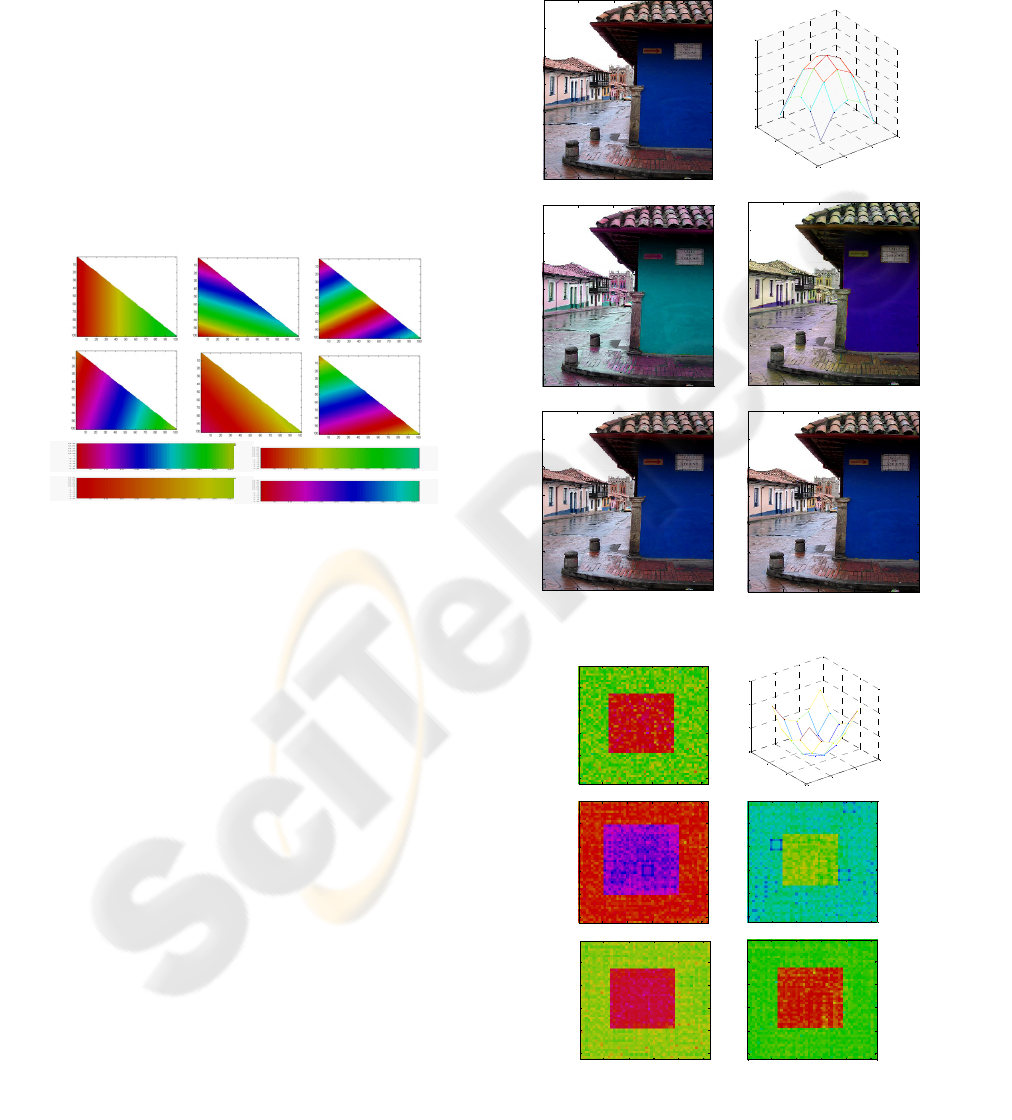
Figure 16: Interpolations of triangles given the vertices red
red green and violet-orange-green; and of lines given
extremes red-citrine and red-cyan.
4.2 Circular Mathematical
Morphology
An alternate way of applying morphological
operators to the hue component of colour images is
to interpret the max and min operators and the
addition operation in the context of a circular
variable, as in Section 2.3. We translate addition as
counter clockwise rotation, i.e. as addition of real
numbers followed by the operation of taking modulo
2π. Then, apply the standard definitions of grey level
image morphology. Occasionally, the data in, say a
3x3 window, have multiple gaps and there is not a
max nor a min, and a special treatment must be
given to the pixel at hand. For this sort of sample,
we choose to leave the corresponding pixels
unchanged.
As can be observed in Figure 17, in the erosion,
the blue of the wall became cyan (a negative shift)
while in the dilation, violet (a positive shift). The red
arrow in a yellowish background grew larger in the
erosion and thinner in the dilation. In Figure 18, two
Von Mises textures are shown; due to the shape of
the structuring element, the inner square grows and
becomes bluer with an erosion; with a dilation, it
shrinks and becomes more yellow; both textures lost
contrast.
Figure 17: Circular morphological operations.
Figure 18: Circular morphological operations.
Original
10 20 30 40 50
10
20
30
40
50
Erosion
10 20 30 40 50
10
20
30
40
50
Dilation
10 20 30 40 50
10
20
30
40
50
Opening
10 20 30 40 50
10
20
30
40
50
Clos ing
10 20 30 40 50
10
20
30
40
50
0
2
4
6
0
2
4
6
0
0.5
1
1.5
Spatial Domain
Structuring Element function
Radians
CIRCULAR PROCESSING OF THE HUE VARIABLE - A Particular Trait of Colour Image Processing
75

5 CONCLUSIONS
We have extended the definition and applied circular
versions of statistics commonly used for linearly
ordered data; in particular, the sample average,
median, gap, min, max, concentration and range. We
applied their running versions as smoothers and edge
detectors of colour images. As expected, for the
noises tried, the median filter works better visually
than the average. We consider that the edge detector
with best performance is the one given by 1-T(gap).
As in the case of the phase of complex numbers,
undeniable useful, in some cases these statistics
must be left undefined. Two methods to apply
morphological operators to angle valued signals are
presented. These novel tools for colour image
processing are likely to be useful.
Unlike previous versions of colour morphology, we
consider only the hue component, leaving the
components of saturation and value unaltered. Also,
we respect the circular nature of the hue variable
while taking advantage of grey level morphology.
The processing of the hue component alone
illustrates the effect of the tools which are particular
due to the circular nature of the hue variable.
The cases of undefined statistics and
morphological operators are more common,
although on a, say 5x5 window, it is probably hard
to find 25 hues uniformly distributed. We have
chosen to leave the corresponding pixels unaltered
but other choices are possible.
We have given algorithms for the interpolation
of hue valued functions on triangular meshes as well
as on 1D discrete domains. We found an unexpected
lack of algorithms for the lifting of angle functions,
this seems to be a fertile field of research.
The field of color image processing is important
in computer vision tasks such as the detection of
malaria in blood films (Ortiz et al., 2005) and also in
tasks where the aesthetic quality of the processed
image is important such as in commercial colour
photography and in digital document restoration.
REFERENCES
Christenson, C.O. and Voxman, W.L., 1998. Aspects of
Topology, BCS Associates, Moscow, Idaho, U.S.A,
2
nd
edition.
Comer, M.L. and Delp, E.J. Morphological Operations for
Colour Image Processing. 1999. Journal of Electronic
Imaging. 8(3), pp. 279-289.
Hanbury, A.G. and Serra, J. Morphological operators on
the unit circle. 2001. IEEE trans. on Image
Processing, vol 10, no. 12, pp. 1842-1850.
Hanbury, A.G. and Serra, J. Mathematical morphology in
the HLS colour space. 2001. Proc. 12
th
BMVC. pp.
451-460.
Heijmans, H.J.A.M., 1994. Morphological Image
Operators, Academic Press, Boston.
Nicolaidis, N. and Pitas, I. Nonlinear processing and
analysis of angular signals. 1998. IEEE trans. on
Signal Processing, vol 46, no. 12, pp. 3181-3194.
Ortiz, M., Pimentel M. y Restrepo, A. Metodología para el
reconocimiento automático de la malaria basada en el
color, 2005. X Simposio de Tratamiento de Señales,
Imagenes y Visión Artificial, Universidad del Valle.
Cali. http://labsenales.uniandes.edu.co.
Peters II, R.A. Mathematical morphology for angle-valued
images. 1997. Proc. SPIE Nonlinear Image Processing
VIII, vol. 3026, pp. 84-94.
Rodríguez, C. and Restrepo, A. Circularidad en los
espacios de color Hering 1 y Hering 2, 2006. XI
Simposio de Tratamiento de Señales, Imagenes y
Visión Artificial, Pontificia Universidad Javeriana,
Bogotá.
Restrepo, A. On colour spaces and on colour perception –
Independence between uniques and chromatic
circularity, 2006. First International Conference on
Computer Vision Theory and Applications, vol. 2,
pp.183-187. Setúbal, Portugal.
Serra, J., 1988. Mathematical Morphology Vol 1,
Academic Press, London.
Vejarano, C. Exploración del uso de la morfología
matemática en en tratamiento de imagenes a color.
2002. Proyecto de grado, Dpt. Ing. Eléctrica y
Electrónica, Universidad de los Andes, Bogotá,
Colombia.
www.higp.hawaii.edu/˜cecily/courses/gg313/DA_book/no
de105.html, 2006.
VISAPP 2007 - International Conference on Computer Vision Theory and Applications
76
