PARAMETERIZED KERNELS FOR SUPPORT VECTOR MACHINE

CLASSIFICATION

Fernando De la Torre and Oriol Vinyals

Robotics Institute, Carnegie Mellon University, Pittsburgh, USA

Keywords:

Visual Learning, Kernel methods, Support Vector Machines, Metric learning.

Abstract:

Kernel machines (e.g. SVM, KLDA) have shown state-of-the-art performance in several visual classiﬁcation

tasks. The classiﬁcation performance of kernel machines greatly depends on the choice of kernels and its

parameters. In this paper, we propose a method to search over the space of parameterized kernels using

a gradient-based method. Our method effectively learns a non-linear representation of the data useful for

classiﬁcation and simultaneously performs dimensionality reduction. In addition, we introduce a new matrix

formulation that simpliﬁes and uniﬁes previous approaches. The effectiveness and robustness of the proposed

algorithm is demonstrated in both synthetic and real examples of pedestrian and mouth detection in images.

1 INTRODUCTION

Kernel methods (Schlkopf and Smola, 2002; Shawe-

Taylor and Cristianini, 2004) are increasingly used for

data clustering, modeling and classiﬁcation problems

because of their state-of-the-art performance, simplic-

ity, and lack of local minima problems. Kernel ma-

chines such as SVM, KPCA, or KLDA project data

into (usually) high dimensional feature spaces, where

linear decision surfaces correspond to non-linear de-

cision surfaces in the original input space. The per-

formance of any kernel machine mostly depends on

the type of kernel and its parameters. The kernel

explicitly deﬁnes a similarity measure between two

samples and implicitly represents the mapping of the

input space to the feature space. In general, differ-

ent problems require different feature spaces, and a

domain-speciﬁc kernel is a useful feature for an algo-

rithm to have. In this paper, we propose a method to

learn a non-linear mapping of the data (i.e. a kernel)

useful to improve classiﬁcation in kernel machines.

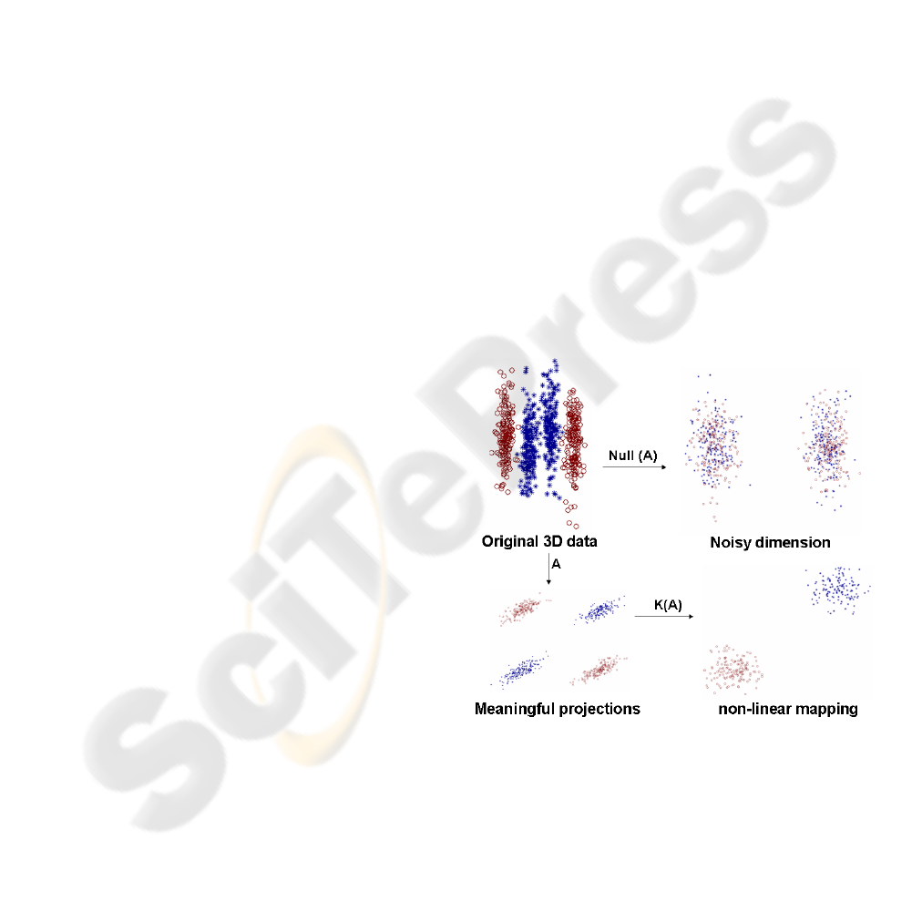
Fig. 1 shows the main point of this paper. We

have synthetically generated 2 multimodal three di-

mensional Gaussian classes. Two of the dimensions

are relevant for classiﬁcation and the other dimension

is high-variance random Gaussian noise. Our algo-

rithm ﬁnds a low dimensional non-linear embedding

Figure 1: Learning a non-linear mapping optimal for classi-

ﬁcation. Top left: original data. Top right: useless features

for classiﬁcation. Bottom left: meaningful projections that

preserve discriminability. Bottom right: ﬁnal non-linear

learned mapping.

of the data where the data is linearly separable. In

this particular example, our algorithm automatically

ﬁnds that the best mapping is a quadratic one, while

discarding the undesirable dimension not relevant for

116

De la Torre F. and Vinyals O. (2007).

PARAMETERIZED KERNELS FOR SUPPORT VECTOR MACHINE CLASSIFICATION.

In Proceedings of the Second International Conference on Computer Vision Theory and Applications - IU/MTSV, pages 116-121

 SciTePress

classiﬁcation. Observe that with a Gaussian kernel

we could achieve similar classiﬁcation performance

in this particular problem (assuming some tuning of

the parameters is done); however, the exponential ker-

nel hides the simplicity of the solution found by our

algorithm (a quadratic mapping).

2 PREVIOUS WORK

Since the introduction of kernel machines in the 90’s,

there has been growing literature on metric and kernel

learning. It is beyond the scope of this paper to review

all previous work along these lines, but a good re-

view on metric learning can be found in (Yang, 2006),

and for kernel selection methods see (Schlkopf and

Smola, 2002; Shawe-Taylor and Cristianini, 2004).

A common approach to learn a kernel matrix uses

semi-deﬁnite programming (SDP) (Lanckriet et al.,

2004; Cristianini et al., 2001) to maximize some sort

of alignment with respect to an ideal kernel. A ma-

jor limitation of SDP is its computational complexity,

since it scales O(n

), where n is the number of sam-

ples (Boyd and Vandenberghe, 2004). This limita-

tion has restricted its application to small scale prob-

lems. Recently, (Kim et al., 2006) posed the ker-

nel selection for kernel linear discriminant analysis

as a convex optimization problem. To optimize over

a positive combination of known kernels, they use

interior point methods with a computational cost of

O(d

+ n

), where d is the dimension of the samples.

Along these lines, (Weinberger et al., 2006) learns a

Mahalanobis distance metric in the kNN classiﬁcation

setting by SDP. The learned distance metric enforces

the k-nearest neighbors to belong to the same class,

while examples from different classes are separated

by a large margin.

In the literature of metric learning, Goldberger et

al. (Goldberger et al., 2004) have proposed Neighbor

component analysis that computes the Mahalanobis

distance that minimizes an approximation of the clas-

siﬁcation error. Similarly, (Shental et al., 2002) opti-

mizes the linear discriminant analysis (LDA) criteria

in a semi-supervised manner to learn the metric.

In previous work, typically, a parameterized fam-

ily of linear or non-linear kernels, (e.g. Gaussian,

polynomial ) are chosen and the kernel parameters are

tuned with some sort of cross-validation. In this pa-

per, we consider the more generic problem of ﬁnding

a functional mapping of the data.

3 PARAMETERIZING THE

KERNEL

Many visual classiﬁcation tasks (e.g. object recogni-

tion) are highly complex and non-linear kernels are

needed to model changes such as illumination, view-

point or internal object variability. Learning a non-

linear kernel is a relatively difﬁcult problem; for in-

stance, proving that a function is a kernel is a chal-

lenging mathematical task. A given function is a

kernel if and only if the value it produces for two

vectors corresponds to a dot product in some feature

Hilbert space. This is the well known Mercer’s the-

orem: ”Every positive deﬁnite, symmetric function

is a kernel. For every kernel K, there is a function

ϕ(x) : k(d

) = hϕ(d

),ϕ(d

)i.”, where hi denotes

dot product. To avoid the problem of proving that a

similarity function is a kernel, it is common to param-

eterize the Kernel as a positive combination of exist-

ing Kernels (e.g. Gaussian, polynomial, ...).

In this paper, we propose to learn a kernel as a pos-

itive combination of normalized kernels as follows:

T = D

T = dm(T)

−

Tdm(T)

−

= D

= dm(T

)

−

dm(T

)

−

(A,α) =

∑

t=0

t

,··· ,A

,α) =

∑

t=0

t

(1)

where α

≥ 0 ∀t, the columns of D ∈ ℜ

d×n

(see nota-

tion

) contain the original data points, d denotes the

dimension of the data, n the number of samples and

p the degree of the polynomial. Each element i j of

the matrix T, t

i j

= d

contains the dot weighted

product between the sample i and j. Each element i j

of the matrix

T represents the cosine of the angle be-

tween the samples i and j (i.e.

i j

k

exponentiates each of the entries in T. K

is a

positive combination of

k

, and if A is positive def-

inite, K

will be a valid kernel because of the closure

Bold capital letters denote a matrix D, bold lower-case

letters a column vector d. d

represents the j column of the

matrix D. d

i j

denotes the scalar in the row i and column

j of the matrix D and the scalar i-th element of a column

vector d

. All non-bold letters will represent variables of

scalar nature. d iag is an operator that transforms a vector

to a diagonal matrix or takes the diagonal of the matrix into

a vector. dm(A) is a matrix that contains just the diagonal

elements of A. ◦ denotes the Hadamard or point-wise prod-

uct. 1

∈ ℜ

k×1

is a vector of ones. I

∈ ℜ

k×k

is the iden-

tity matrix. tr(A) =

∑

is the trace of the matrix A and

|A| denotes the determinant. ||A||

= tr(A

A) designates

the Frobenious norm of a matrix. A

k

denotes point-wise

power, i.e. a

i j

∀i, j.

PARAMETERIZED KERNELS FOR SUPPORT VECTOR MACHINE CLASSIFICATION

117

properties of kernels (Shawe-Taylor and Cristianini,

2004). The rank of each of the matrices

T and

min{d,n}, but K

might be full rank. The same in-

terpretation holds for K

with the difference that for

each kernel

there is a different metric matrix A

that is, each kernel might have a different subspace to

project the data onto. The matrix A

models correla-

tions between variables.

The kernel expansion suggested in eq. 1 is, in

spirit, similar to the Taylor series expansion of a mul-

tivariate function. In fact, K

and K

can represent

directly the polynomial kernel and are closely related

to the exponential one. Consider a set of normalized

samples (i.e.

= d

/||d

), the Taylor series expan-

sion of two elements of the exponential kernel will be

i j

= e

−

∑

∞

i=0

(2)

(1 −

)

, which has an

identical form of the expansion proposed in eq. 1 if

= I

∀t. Observe that our kernel expansion is more

ﬂexible and it will learn a mapping useful for classi-

ﬁcation from training data. However, K

and K

are

not translational invariant kernels.

3.1 Dealing with High Dimensional

Data

For high dimensional data (e.g. images) A ∈ℜ

d×d

a big matrix that captures the correlation relation be-

tween the features. In our context, working with these

very high dimensional matrices presents two prob-

lems: computational tractability (storage, efﬁciency

and rank deﬁciency) and generalization.

In order to be able to generalize better and to not

suffer from storage/computational limitations, we fol-

low recent work (de la Torre and Kanade, 2005) and

factorize the matrix A as a low dimensional subspace

plus a noisy term (scaled identity matrix). That is,

we approximate each matrix A

as A

≈ B

+ λ

where λ

≥ 0 ∈ ℜ and B

∈ ℜ

d×k

. It is worthwhile to

point out two important aspects of the previous fac-

torizations. Factorizing the covariance as the sum of

outer products and a diagonal matrix is an efﬁcient

(in space and time) manner to reduce the dimension-

ality of the data. Firstly, observe that to compute

≈B(B

)+λd

storing/computing the full d ×d

covariance is not required. Secondly, the original ma-

trix A has d(d + 1)/2 free parameters, and after the

factorization the number of parameters is reduced to

k(2d −k + 1)/2 (assuming orthogonality of B), and

hence is not so prone to over-ﬁtting.

4 LEARNING FROM AN IDEAL

KERNEL

In the previous section, we have proposed a possi-

ble expansion of a parameterized kernel. Ideally, we

would like to directly optimize the kernel parameters

to minimize the Bayes classiﬁcation error; however,

this is usually a hard task because the underlying dis-

tribution of the data is unknown and usually some sort

of bounds are optimized instead. In this section, we

explore the use of a ideal reference kernel to learn the

kernel parameters.

In the ideal case, we would like to estimate the

parameters of the kernel (A,α) to produce a block di-

agonal matrix (assuming samples are ordered). That

is, in all the samples that belong to the same class the

kernel function should output a similarity of 1 and 0

otherwise. This ideal matrix can be computed with

the matrix G as F = GG

. A reasonable measure of

distance between the ideal kernel and the parameter-

ized one is given by:

(A,α) = ||F −K(A,α)||

∝

tr(K(A,α)K(A,α)

) −2tr(K(A,α)F) (2)

This measure of distance between kernels is

closely related to the one proposed by (Cristianini

et al., 2001). Cristianini et al. propose to mini-

mize the alignment between kernels with: E

(A,α) =

tr(K(A,α)F)

√

tr(K(A,α)K(A,α))

. Minimization of E

is more

convenient to optimize and very similar (but not

equivalent) to maximization of E

. Recall that if

we take the log E

and change the sign, E

∝

0.5log(tr(K(A,α)

)) −logtr (K(A, α)F).

One drawback of eq. 2 is that it enforces the same

similarity measure (i.e. 1) for two samples of the

same class that are near or far away in the input space.

This behavior can produce over-ﬁtting and it can re-

move important information regarding class discrim-

inability. Moreover, we can have an unbalanced prob-

lem where a particular class has more samples than

another one, and we would like a mechanism to com-

pensate for that. Furthermore, any real data set con-

tains a number of outliers that can bias the solution.

To account for these situations, we introduce a new

distance matrix W ∈ ℜ

n×n

that will weight individ-

ually each pair-wise points. For instance, to account

for outliers we will weight all the rows and columns

of the outlying data as 0, or to compensate for the fact

that two samples have large dissimilarity in the input

space, we enforce a small link between these samples

e.g w

i j

= e

−

||d

−d

∀i 6= j. To incorporate W in the

VISAPP 2007 - International Conference on Computer Vision Theory and Applications

118

formulation, we modify eq. 2 as:

(A,α) = ||W ◦(F −K(A,α))||

∝

tr((W ◦K(A,α))(K(A,α) ◦W)

)

−2tr((W ◦K(A,α))(W ◦F)) (3)

5 LEARNING THE KERNEL

In this section, we derive several optimization strate-

gies to learn a parameterized kernel.

5.1 Optimizing w.r.t A and α

In the interest of space, we derive the optimization

rules for the most generic error function. In particular,

we show how to optimize:

,··· ,A

,α) = ||W ◦(F −K

)||

(4)

w.r.t. A

,··· ,A

,α, since optimizing K

is very sim-

ilar. To optimize eq. 4, we use an alternating strat-

egy of ﬁxing A

parameters and optimize w.r.t. α and

vice versa. This will monotonically decrease the error

of E

. If α is known, optimizing over A

matrix can

be formulated as a semi-deﬁnite programming prob-

lem (SDP); however, the computational complexity is

large. Instead, we use a gradient descent approach to

incrementally optimize for A

. The gradient updates

are given by:

n+1

= A

−η

∂E

)

∂A

(5)

∂E

∂A

= 2α

tD(M

−M

∀t

= (K

−F) ◦

(t−1)

◦W

2

= dm(T

)

−

dm(T

)

−

= dm(T

)

−

diag



(dm(T

)

−

◦T



The major problem with the update of eq. 5 is to

determine the optimal η. In our case, η is determined

with a line search strategy (Fletcher, 1987). Similarly,

for high dimensional data the gradient w.r.t B

is:

n+1

= B

−η

∂E

)

∂B

(6)

∂E

∂B

= 2α

tD(M

−M

∀t

At this point, it is worthwhile to mention that the com-

plexity of the updates is O(d + n

), far less expensive

than SDP approaches. λ

is optimized using the fmin-

con function from Matlab

 to ensure positiveness.

Once all A

∀t have been updated, α values can be

optimized using quadratic programming. After rear-

ranging, eq. 4 can be expressed as:

(α) ∝ α

Zα −2p

α α ≥0 (7)

where z

i j

∑

and p

∑

. Re-

call that k

i j

corresponds to the i j element of K

. We

use the quadprog function from Matlab

 to opti-

mize w.r.t.α to ensure positiveness.

5.2 Initialization and Other Issues

Minimizing eq. 4 w.r.t to α, A

,··· ,A

is a non-

convex optimization problem prone to many local

minima. Without a good initial estimation, the pre-

vious optimization scheme easily converges to a local

minima. To get a reasonable estimation, we initial-

ize each of the parameters A

,··· ,A

with the LDA

solution and the means of the clusters resulting from

k-means clustering. The α values are initialized with

the same uniform value. Moreover, we start from sev-

eral random initial points and select the solution with

minimum error after convergence.

To avoid over-ﬁtting problems and for computa-

tional convenience, we train the algorithm stochasti-

cally. That is, we randomly select subsets of training

data, run few iterations of the gradient descent algo-

rithm, select other random subset of data and proceed

this way until convergence.

6 EXPERIMENTS

In this section, we report comparative results of our

algorithm with standard SVM approaches in image

classiﬁcation problems. In all the experiments we

have used the C-SVM implementation (Chang and

Lin, 2001).

6.1 Synthetic Data

Consider ﬁg. 1, where 200 samples have been gener-

ated from four 3D Gaussians (50 each) from 2 differ-

ent classes (”exclusive or” (XOR) problem). For each

of the Gaussians, the z coordinate is random noise of

high variance.

In this case, we learn a common matrix A ∈ ℜ

3×3

and the α values. After convergence, the rank of the

matrix A is 3 with eigenvalues l

= 1.9860 l

0.6843 l

= 0.0009, the small eigenvalue corre-

sponds to the eigenvector aligned with the z direc-

tion, where the non-discriminative information lies.

That is, the null space of A contains the random non-

discriminative directions. Even more interesting is the

interpretation of the α parameters. All the α param-

eters are close to 0 except for the powers of 2. This

is because, for samples within the same cluster, the

cosine of the angle will be approximately 1; between

the samples of a different cluster but of the same class

PARAMETERIZED KERNELS FOR SUPPORT VECTOR MACHINE CLASSIFICATION

119

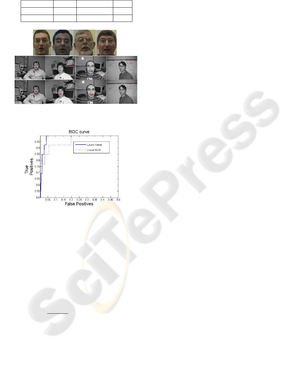
Table 1: Average classiﬁcation results for different kernels.

Features Linear Exponential Ours

Graylevel 73.9 76.4 84.2

Multiband 72.4 79.1 84.9

Figure 5: a) Some training examples of the IBM Database.

b) First row the same images with our learned kernel (3/3).

Second row some test images using the RBF SVM (1/3).

Figure 6: Roc curves of RBF versus our algorithm.

possible locations of the image. Evaluating the kernel

at each location (x, y) can be computationally expen-

sive. For a particular position (x,y) computing the

projection B

is equivalent to correlating the im-

age with each basis of the subspace B

, and stacking

all the values for each pixel. For large regions, this

correlation is performed efﬁciently in the frequency

domain using the Fast Fourier Transform (FFT) (i.e.

= b

I = IFFT (FFT (b

) ◦FFT (I))). This fast

search is another advantage of our formulation. Fig. 6

shows the average ROC curve over 14 images for our

kernel and RBF kernel. The parameters of the RBF

kernel (i.e. e

−||x

−x

2σ

, σ and the C in the C-SVM

are tuned with a cross validation procedure. Similarly

the C parameter in the C-SVM is tuned with cross-

validation. Fig. 5.b shows some examples of the

detection performance of the RBF-SVM versus our

learned kernel. In the ﬁrst row, our learned kernel de-

tects two out of three mouths, whereas in the second

row RBF only detects one.

ACKNOWLEDGEMENTS

The work was partially supported by grants from

the National Institute of Justice (award 2005-

IJ-CX-K067) and Defense Advanced Research

Projects Agency (DARPA) under Contract No.

NBCHD030010. Thanks to Minh Hoai Ngyen for

helpful discussions and comments.

REFERENCES

Boyd, S. and Vandenberghe, L. (2004). Convex Optimiza-

tion. Cambridge University Press.

Chang, C.-C. and Lin, C.-J. (2001). LIBSVM: a library

for support vector machines. Software available at

http://www.csie.ntu.edu.tw/ cjlin/libsvm.

Cootes, T. F. and Taylor, C. J. (2001). Statistical

models of appearance for computer vision. In

http://www.isbe.man.ac.uk/bim/refs.html.

Cristianini, N., Taylor, J. S., and Elisseeff, A. (2001). On

kernel-target alignment. In NIPS.

de la Torre, F. and Kanade, T. (2005). Multimodal oriented

discriminant analysis. In ICML.

Fletcher, R. (1987). Practical methods of optimization. John

Wiley and Sons.

Goldberger, J., Roweis, S., Hinton, G., and Salakhutdinov,

R. (2004). Neighbourhood component analysis. In

NIPS, pages 513–520.

Kim, S.-J., Magnani, A., and Boyd, S. (2006). Optimal

kernel selection in kernel ﬁsher discriminant analysis.

In ICML, pages 465–472.

Lanckriet, G., Cristianini, N., Bartlett, P., Ghaoui, E., and

Jordan, M. (2004). Learning the kernel matrix with

semideﬁnite programming. (5):27–72.

Munder, S. and Gavrilla, D. (2006). An experimental study

on pedestrian classifcation.

Neti, C., Potamianos, G., Luettin, J., Matthews, I., Glotin,

H., Vergyri, D., Sison, J., Mashari, A., and Zhou,

J. (2000). Audio-visual speech recognition. Tech-

nical Report WS00AVSR, Johns Hopkins University,

CLSP.

Schlkopf, B. and Smola, A. (2002). Learning with Kernels:

Support Vector Machines, Regularization, Optimiza-

tion, and Beyond. MIT Press.

Shawe-Taylor, J. and Cristianini, N. (2004). Kernel Meth-

ods for Pattern Analysis. Cambridge university press.

Shental, N., Hertz, T., Weinshall, D., and Pavel, M. (2002).

Adjustment learning and relevant component analysis.

In European Conferenceon Computer Vision, pages

776–790.

Weinberger, K., Blitzer, J., and Saul, L. (2006). Neighbour-

hood component analysis. In NIPS.

Yang, L. (2006). Distance metric leraning: A comprehen-

sive survey.

PARAMETERIZED KERNELS FOR SUPPORT VECTOR MACHINE CLASSIFICATION

121