MODELING NON-GAUSSIAN NOISE FOR ROBUST IMAGE

ANALYSIS

Sio-Song Ieng

ERA 17 LCPC, Laboratoire des Ponts et Chauss

ees, 23 avenue de l’amiral Chauvin, B.P. 69, 49136 Les Ponts de C

e, France

Jean-Philippe Tarel

ESE, Laboratoire Central des Ponts et Chauss

ees, 58 Bd Lefebvre, 75015 Paris, France

Pierre Charbonnier

ERA 27 LCPC, Laboratoire des Ponts et Chauss

ees, 11 rue Jean Mentelin, B.P. 9, 67035 Strasbourg, France

Keywords:

Image Analysis, Statistical Approach, Noise Modeling, Robust Fitting, Image Grouping and Segmentation,

Image Enhancement.

Abstract:

Accurate noise models are important to perform reliable robust image analysis. Indeed, many vision prob-

lems can be seen as parameter estimation problems. In this paper, two noise models are presented and we

show that these models are convenient to approximate observation noise in different contexts related to image

analysis. In spite of the numerous results on M-estimators, their robustness is not always clearly addressed

in the image analysis ﬁeld. Based on Mizera and M

uller’s recent fundamental work, we study the robustness

of M-estimators for the two presented noise models, in the ﬁxed design setting. To illustrate the interest of

these noise models, we present two image vision applications that can be solved within this framework: curves

ﬁtting and edge-preserving image smoothing.

1 INTRODUCTION

In computer vision, it is common knowledge that

data are corrupted by non-Gaussian noise, outliers

and may contain multiple statistical populations. It

is a difﬁcult task to model observed perturbations.

Several parametric models were proposed in (Huang

and Mumford, 1999; Srivastava et al., 2003), and

sometimes based on mixtures (Hasler et al., 2003).

Non-Gaussian noise models imply using robust al-

gorithms to reject outliers. The most popular tech-

niques are Least Median Squares (LMedS), RANSAC

and Iterative Reweighted Least Squares (IRLS). The

first two algorithms are close in their principle and

achieve the highest breakdown point, i.e. the admis-

sible fraction of outliers in the data set, of approx-

imately 50%. However, their computational burden

quickly increases with the number of parameters. In

this paper, we focus on the IRLS algorithm, which is

an extension of least-squares allowing non-Gaussian

noise models, see (Huber, 1981). IRLS means Iter-

ative Reweighted Least-Squares, where the weight λ

is a particular function of the noise model at the value

of the residual. One may argue that IRLS algorithm is

a deterministic algorithm that only converges towards

a local minimum close to its starting point. This dif-

ﬁculty can be circumvented by the so-called Gradu-

ated Non Convexity (GNC) strategy. The IRLS algo-

rithm, even with the GNC strategy, is usually very fast

compared to LMedS and RANSAC and it also able to

achieve the highest breakdown point.

Indeed, let us consider the linear problem:

Y = XA+ B (1)

where Y = (y

,···,y

) ∈ R

is a vector of observa-

tions, X = (x

,···,x

) ∈ R

n×d

the design matrix, A ∈

the vector of unknown parameters that will be esti-

mated by the IRLS algorithm, and B = (b

,···,b

) ∈

the noise. The noise is assumed independent and

identically distributed but not necessarily Gaussian.

We consider the ﬁxed design setting, i.e. in (1), X is

assumed non-random. In that case, as demonstrated

in (Mizera and M

uller, 1999), certain M-estimators

attain the maximum possible breakdown point. How-

ever, if X cannot be assumed non-random, the break-

down point of M-estimators drops towards zero (Meer

et al., 2000). This underlines how important the way

computer vision problems are formulated is. To our

183

Ieng S., Tarel J. and Charbonnier P. (2007).

MODELING NON-GAUSSIAN NOISE FOR ROBUST IMAGE ANALYSIS.

In Proceedings of the Second International Conference on Computer Vision Theory and Applications - IFP/IA, pages 183-190

 SciTePress

opinion, many problems can be expressed in the fixed

design setting, allowing to apply the fast and efﬁcient

IRLS algorithm.

The paper is organized as follows. In Sec. 2,

we present the non-Gaussian noise models we found

of interest in diverse contexts, which is shown in

Sec. 3. Then in Sec. 4, we prove that M-estimators

that achieve the maximum breakdown point of ap-

proximately 50% can be built based on these proba-

bility distribution families. Finally in Sec. 5, we illus-

trate the interest of these theoretical results, by pre-

senting two applications, casted in the fixed design

setting: curves ﬁtting for lane-marking shape estima-

tion and edge-preserving image smoothing.

2 NON-GAUSSIAN NOISE

MODELS

We are interested in parametric functions families that

allow a continuous transition between different kinds

of probability distributions. We here focus on two

simple parametric probability density functions (pdf)

of the form pd f (b) ∝ e

−ρ(b)

suitable for the IRLS al-

gorithm, where ∝ denotes the equality up to a factor.

A first interesting family of pdfs is the exponential

family (also called generalized Laplacian, or gener-

alized Gaussian, or stretched exponential (Srivastava

et al., 2003)):

α,s

(b) =

sΓ(

2α

)

−((

)

(2)

The two parameters of this family are the scale s and

the power α, which specifies the shape of the noise

model. Moreover, α allows a continuous transition

between two well-known statistics: Gaussian (α = 1)

and Laplacian (α =

). The associated ρ function is

(b) = ((

)

As detailed in (Tarel et al., 2002), to guarantee

the convergence of IRLS,

′

(b)

has to be deﬁned on

[0,+∞[, which is not the case for α ≤ 0 in the expo-

nential family. Therefore, the so-called smooth ex-

ponential family (SEF) S

α,s

was introduced in (Ieng

et al., 2004):

α,s

(b) ∝

−

(

)

(3)

where ρ

(u) =

((1+ u

)

−1).

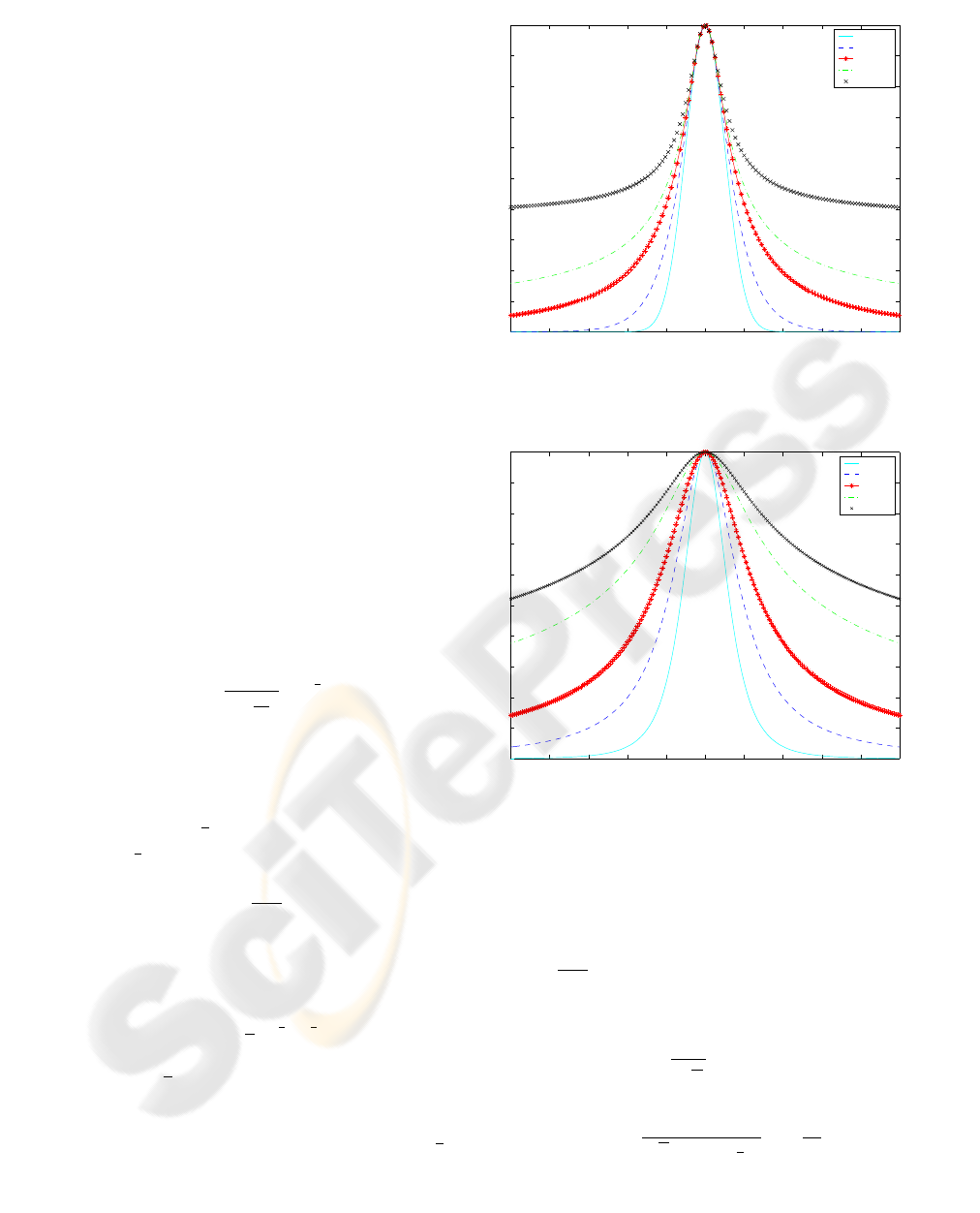
Similarly to the exponential family, α allows a

continuous transition between well-known statistical

laws such as Gauss (α = 1), smooth Laplace (α =

)

and Geman & McClure (α = −1). These laws are

shown in Figure 1. For α ≤0, S

α,s

can be always nor-

malized on a bounded support, so it can still be seen

−10 −8 −6 −4 −2 0 2 4 6 8 10

0.1

0.2

0.3

0.4

0.5

0.6

0.7

0.8

0.9

α,s

distribution

α = 1

α = 0.5

α = 0.1

α = −0.1

α = −0.5

Figure 1: SEF noise models, S

α,s

. Notice how tails are

getting heavier as α decreases.

−10 −8 −6 −4 −2 0 2 4 6 8 10

0.1

0.2

0.3

0.4

0.5

0.6

0.7

0.8

0.9

β = 2

β = 1

β = 0.6

β = 0.3

β = 0.2

Generalized T−Student Distributions

Figure 2: GTF noise models, T

β,s

. Notice how tails are

getting heavier when β is increasing towards 0.

as a pdf. In the smooth exponential family, when α

is decreasing, the probability to have large, not to say

very large errors (outliers) increases.

In the IRLS algorithm, the residual b is weighted

by λ =

′

(b)

. Notice that while the pdf is not defined

when α = 0, its weight does and it corresponds in fact

to the T-Student law. Moreover, it is easy to show

that the so-called generalized T-Student pdfs have the

same weight function

up to a factor. We define

the Generalized T-Student Family (GTF) by:

β,s

(b) =

Γ(−β)

√

πΓ(−β−

(1+

)

(4)

where β < 0. This family of pdfs also satisﬁes the re-

quired properties for robust ﬁtting. It is named gener-

alized T-Student pdf (Huang and Mumford, 1999) in

the sense that an additional scale parameter is intro-

duced compared to the standard T-Student pdf. No-

tice, that the case β = −1 corresponds to the Cauchy

pdf. These laws are shown in Figure 2. The GTF can

be rewritten as:

β,s

(b) ∝

−

(b)

(5)

where ρ

(b) = −2βlog(1+

The parameters of the GTF are s and β (β < 0).

They play exactly the same role as s and α in the SEF.

For −

≤β < 0, as previously the pdf is defined only

for a bounded support.

3 IMAGE NOISE MODELING

We have used with success SEF and GTF for noise

modeling in different image analysis applications. We

now illustrate this on two particular examples, where

geometric and photometric perturbations are consid-

ered in turn, and modeled using the smooth exponen-

tial family (SEF).

3.1 Geometry

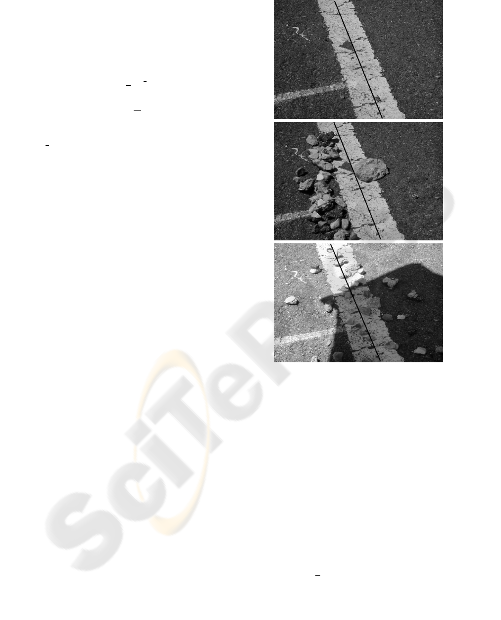
In this experiment, we have taken a set of 150 im-

age of the same marking with different perturbations

such as stones, shadows and so on, see Figure 3. The

ground-truth position of the lane marking center was

obtained by hand. It is shown in black in Figure 3.

Then, for each of these images, local marking cen-

ters are extracted, see (Ieng et al., 2004) for details,

and the horizontal distances to each feature center

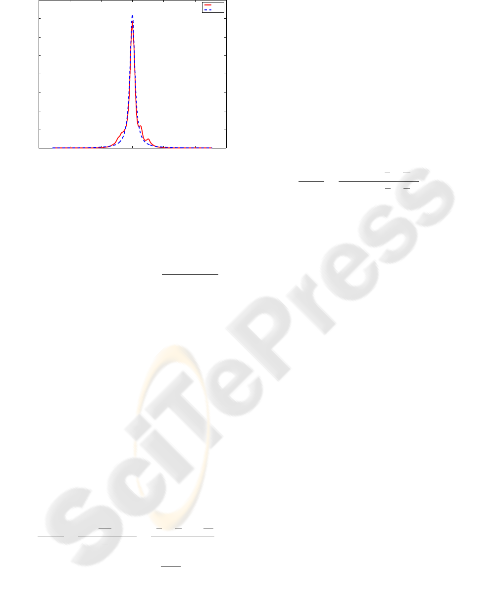
with respect to the reference are collected. The MLE

approach is then applied to estimate α and s at the

same time by a non-linear minimization with a gra-

dient descent. The best parameters within SEF are

α = 0.05 and s = 1.1. As shown in Figure 4, these

parameters seems to lead to a nice noise model.

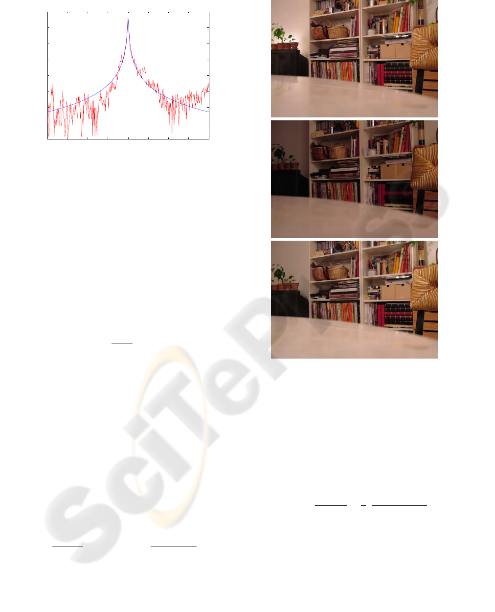
3.2 Photometry

We performed a similar experiment for photometric

information. We have taken a set of 19 images of the

same scene with different light conditions as shown

on Fig 5. The ground truth is not easy to build con-

trary to the previous section. As a consequence, we

compute, for each pair of images, the histogram of

the differences in intensity between the two images,

for each pixel. Rather than to sample the pdf of the

perturbations, we sample the autocorrelation function

of the pdf.

Figure 3: Three of the 150 images of the same marking

with different perturbations. The black straight line shows

the reference marking position.

After ﬁtting of the SEF model, we obtained a

quite accurate model of the autocorrelation function

as shown in Fig 6, with α = 0.02 and s = 9.

4 ROBUSTNESS STUDY

Following (Mizera and M

uller, 1999), in the fixed de-

sign case, robustness of an M-estimator is character-

ized by its breakdown point which is deﬁned as the

maximum percentage of outliers the estimator is able

to cope with:

∗

(

A,Y,X) =

min{m : sup

Y∈B(Y,m)

Y,X)k= ∞}

(6)

where

Y is a corrupted data set obtained by arbitrary

changing at most m samples, B is the set of all

−200 −150 −100 −50 0 50 100 150 200

−10

−9

−8

−7

−6

−5

−4

−3

−2

Log histogram fit

residual

log(probability)

Figure 4: Log histogram of the residual errors in feature

centers collected from 150 images after local marking ex-

traction. The obtained distribution is well approximated by

the best fit SEF (3) with parameters α = 0.05 and s = 1.1.

B(Y,m) = {

Y : card{k : ˜y

6= y

} ≤ m} and

Y,X)

is an estimate of A from

Y. It is important to notice

that the previous deﬁnition is different from the one

proposed in (Hampel et al., 1986) which is not suited

to the fixed design setting.

Mizera and M

uller (Mizera and M

uller, 1999) also

emphasize the notion of regularly varying functions,

and described the link between this kind of regular-

ity and robustness property. By deﬁnition, f varies

regularly if there exists a r such that:

lim

t→∞

f(tb)

f(t)

= b

(7)

When the exponent r equals zero, the function is said

to vary slowly, i.e. the function is heavily tailed.

We now assume that the ρ function of the M-

estimator follows the four following conditions:

1. ρ is even, non decreasing on R

and nonnegative,

2. ρ is unbounded,

3. ρ varies regularly with an exponent r ≥0,

4. ρ is sub-additive: ∃L > 0, ∀t,s ≥ 0, ρ(s + t) ≤

ρ(s) + ρ(t) + L.

The main result proved in (Mizera and M

uller,

1999) is that the percentage ε

∗

is bounded by a func-

tion of r:

Theorem. Under the four previous conditions on ρ,

and if r ∈ [0, 1], then ∀Y and X,

M(X,r)

≤ ε

∗

(

A,Y,X) ≤

M(X,r) + 1

(8)

where, with the convention 0

= 0, M(X,r) is defined

as:

M(X,r) = min

A6=0

{card(K) :

∑

k∈K

≥

∑

k/∈K

}

(9)

Figure 5: Three of the 19 images of the same scene with

different lighting conditions.

where K runs over the subsets of {1,2,···,n}.

When the exponent r is zero, the exact value of the

percentage ε

∗

is known. The following theorem states

its value.

Theorem. Under the four previous conditions on ρ

and if r = 0, then ∀ Y and X,

∗

(

A,Y,X) =

M(X,0)

⌊

n−

N (X) + 1

⌋ (10)

where ⌊x⌋ represents the integer part of x, and

N (X) = max

A6=0

{card{X

: X

A = 0}, k = 1,···,n}.

This value is also the maximum achievable value

which is approximatively 50%. As a consequence, M-

estimators with zero r exponent are of highest break-

down point.

Finally in (Mizera and M

uller, 1999), it is shown

that the bounds on the percentage ε

∗

are related to r as

−300 −200 −100 0 100 200 300

0.005

0.01

0.015

0.02

0.025

0.03

0.035

0.04

Intensity

pdf

data

fit

Figure 6: Histogram of the intensity differences collected

from 19 images. The obtained distribution is well approxi-

mated by the best fit SEF (3) with parameters α = 0.02 and

s = 9.

a decreasing function. This is stated by the following

lemma:

Lemma. If q ≥ r ≥ 0 then

M(X,q) ≤ M(X,r) ≤ M(X,0) = ⌊

n−

N (X )+ 1

⌋.

With these three results, the relationship between

the exponent r of the function ρ and the robustness

of the associated M-estimator was clearly established.

As a consequence of these important theoretical re-

sults, the robustness of a large class of M-estimators

can be compared just by looking at the exponent r of

the cologarithm of their associated noise pdf. To illus-

trate this, we now apply the above results to the SEF

and GTF pdfs described in Sec. 2.

4.1 The SEF Case

Let us prove that the robustness of SEF based M-

estimators is decreasing with α ∈]0,0.5]. To this end,

we first check the four above conditions on the ρ

function. Function ρ

is clearly even, non decreasing

on R

and nonnegative. The first condition is thus

satisﬁed. The second one is fulﬁlled only when α > 0,

due to the fact that ρ

is bounded for α ≤0. Looking

at the ratio:

(tb)

(t)

(1+

)

−1

(1+

)

−1

(

)

−

2α

(

)

−

2α

we see that when α > 0, lim

t→∞

(tb)

(t)

= b

2α

. As

a consequence, the ρ

function varies regularly and

the third condition is also satisﬁed. For the fourth

condition, we can use Huber’s Lemma 4.2 (Huber,

1984), to prove the sub-additivity when α ∈]0,0.5[.

For α = 0.5, it can also be proved that ρ

is sub-

additive. All conditions on ρ being fulﬁlled, the first

Theorem applies, and using the Lemma, we prove that

the robustness of SEF M-estimators is increasing to-

wards the maximum of approximatively 50%, with re-

spect to a decreasing α parameter within ]0,0.5].

4.2 The GTF Case

Let us prove that the robustness of GTF M-estimators

is maximum, whatever the value of β. We shall first

check the 4 conditions on the associated ρ function.

The first two assumptions are easy to check for ρ

Looking at the ratio:

(tb)

(t)

ln(t

) + ln(

))

ln(t

) + ln(

))

we deduce: lim

t→∞

(tb)

(t)

= 1 = b

. As a conse-

quence, the ρ

function varies slowly, and the third

condition is fulﬁlled. The fourth condition is proved

by using Huber’s Lemma 4.2 (Huber, 1984). All

conditions on ρ being satisﬁed, the second Theorem

applies, showing that GTF M-estimators achieve the

highest breakdown point of approximately 50%.

5 APPLICATIONS

We now describe two applications showing how in-

teresting the use of SEF or GTF is in applying robust

algorithms to problems related to geometry and pho-

tometry.

5.1 Curve Fitting for Lane-marking

Tracking

This application is detailed in (Tarel et al., 2002; Ieng

et al., 2004). The problem of tracking a lane mark-

ing can be handled using Kalman ﬁltering, if the lane

marking is robustly ﬁtted in each image, which can

be cast in the linear framework (1). In that case,

A = (a

,··· ,a

) are the parameters of a curve within

a linearly parameterized family: y =

∑

j=1

(x).

The road shape features (x

) are given by the lane-

marking centers extracted using a local feature ex-

tractor (Ieng et al., 2004). In (1), the noisy obser-

vations are the y

. The vector x

= ( f

))

j=1,···,d

is assumed non random. The problem is thus set

in the fixed design and maximum robustness can be

achieved by modeling the geometric noise using the

GTF family. Within the GTF family, the IRLS algo-

rithm is used several time to reﬁne the curve ﬁtting

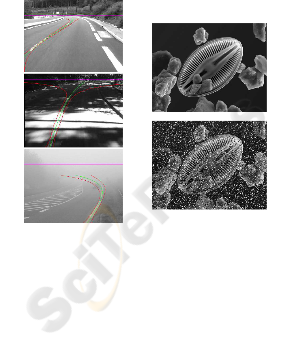
Figure 7: Three examples of detected lane-marking of de-

gree 3 (in green). The uncertainty about the lane-marking

location are also shown (in red).

result with decreasing scale s, until the scale of the

noise is reached. The initial solution is obtained with

a scale large enough to imply a convex minimization

problem. The SEF family can also be used if it bet-

ter corresponds to the observed noise. In such a case

rather than to decrease the scale, we reﬁne the curve

ﬁtting by decreasing α step-by-step until the α of the

observed noise is achieved. The initial solution is ob-

tained with α = 0.5 where the minimization problem

is convex. These two strategies are examples of the

GNC strategy.

Finally, the IRLS, with GNC strategy, allows

curve tracking in real time, contrary to other robust

methods such as LMedS and RANSAC. Three exam-

ples of main curve detection and tracking are shown

in Fig. 7.

5.2 Edge-Preserving Image Smoothing

(a)

(b)

Figure 8: The original image (a), perturbated with 20% salt

and pepper noise (b) (PSNR=11.5dB).

Image smoothing is an important topic in image anal-

ysis. Figure 8 shows an original image and the same

image perturbated with photometric salt and pepper

noise. As is well-known, using classical Gaussian ﬁl-

tering degrades edges, as shown in Figure 9(a). This

motivated many works on nonlinear ﬁltering (Astola

and Kuosmanen, 1997) and edge-preserving image

smoothing, see e.g. (Kervrann and Boulanger, 2006)

for more references. In particular, bilateral ﬁlter-

ing (Tomasi and Manduchi, 1998) is very intuitive be-

cause it is only a generalization of Gaussian smooth-

ing that takes into account both spatial and intensity

variations in the vicinity of each pixel. In (Elad,

2002; Kervrann, 2004), the bilateral ﬁltering theoret-

ical background is explained which opens the possi-

bility of using high breakdown point M-estimators de-

rived from SEF and GTF noise models. Indeed, bilat-

eral ﬁltering can be seen as a linear estimation prob-

lem Y = A + B where Y is the observed image, A is

the source image and B is the noise. Thus, bilateral

ﬁltering can be set as in (1) within the fixed design.

Let us consider a particular pixel (i, j). Its ob-

served intensity is y

i, j

, and a

i, j

is the noiseless inten-

sity that is to be estimated over a square neighbor-

hood [i −m,i + m] ×[ j −m, j + m], assuming a non-

Gaussian noise. To this end, the following error crite-

rion is minimized:

e(a

i, j

) =

∑

k=−m

∑

l=−m

ρ(a

i, j

−y

i+k, j+l

)k(k,l) (11)

where ρ characterizes the noise model along inten-

sities and k is a decreasing function w.r.t. the dis-

tance to the origin. This k allows to take into ac-

count the spatial distribution of the pixels and most

of the time, a Gaussian kernel is used (Tomasi and

Manduchi, 1998). One iteration of bilateral ﬁltering

directly consists of applying the IRLS algorithm de-

rived from (11), for each image pixel.

In (Tomasi and Manduchi, 1998; Elad, 2002;

Kervrann, 2004), it is suggested to use functions from

the M-estimator theory, for ρ. ρ

is an interesting

candidate because it allows continuous transition be-

tween different kinds of pdfs, with increasing robust-

ness when α decreases. Figure 9 displays the re-

sults obtained on the noisy image shown in Figure 8

for bilateral ﬁltering with SEF and different values

of α. When α = 1, the obtained ﬁlter is equivalent

to a weighted mean with Gaussian weights. When

α = 0.5, ρ(x) approximates |x| and hence, the ﬁlter

behaves as a spatially-weighted median ﬁlter. As can

be seen on Figure 9, the lower the value of α, the bet-

ter the restauration quality. However, when α < 0.5,

becomes non-convex and the estimator can get

stuck in a local minimum, resulting in poor results as

show on Figure10(a).

Similarly to (Kervrann, 2004) where the scale pa-

rameter is decreased regularly, we propose to decrease

α step-by-step in a continuation strategy. This is an-

other illustration of the effectiveness of the GNC strat-

egy, see Figure 10(b).

6 CONCLUSION

In this paper, we applied Mizera and M

uller’s funda-

mental work on M-estimators breakdown point cal-

culation in the field of image analysis. In the ﬁxed

design setting, they shown that certain M-estimators

can achieve maximum robustness. Using their re-

sults, we discussed the robustness of M-estimators

based on two non-Gaussian pdfs families, that we in-

troduced under the names of SEF and GTF. In par-

ticular, we shown that the GTF noise model leads to

(a)

(b)

(c)

Figure 9: On the noisy image in Figure 8(b), a bilat-

eral ﬁltering is applied with different values of α within

SEF: Gaussian-weighted mean ﬁltering in (a) with α = 1

(PSNR=20.3dB), α = 0.75 in (b) (PSNR=25.2dB), and

equivalent to weighted median ﬁltering in (c) with α = 0.5

(PSNR=28.1dB). Notice how results are improved when α

decreases.

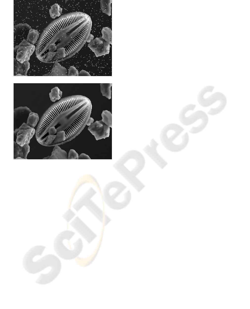
(a)

(b)

Figure 10: The result after bilateral ﬁltering with SEF and

α = 0.25 is in (a) (PSNR=19.6dB). Outliers sill remains due

to the fact that the corresponding ρ function is non convex.

However, a better result is obtained in (b) using GNC strat-

egy (PSNR=28.1dB).

M-estimators that achieve the maximum breakdown

point of approximately 50%, and that the robustness

associated with SEF increases towards the maximum

as α decreases towards 0.

In the second part of this paper, we illustrated how

useful these results are in the context of image analy-

sis: SEF and GTF approximate models seems to cor-

rectly fit observed noise pdfs in diverse applications

and contexts. Moreover, many image analysis prob-

lems can be seen as parametric estimation or cluster-

ing. In the applications we shown (curve ﬁtting and

edge-preserving image smoothing), we observed the

advantage of varying the noise model, progressively

introducing robustness, with the so-called GNC strat-

egy. We therefore believe that the SEF and GTF fam-

ilies can also be used with advantages in many other

image analysis algorithms.

REFERENCES

Astola, J. T. and Kuosmanen, P. (1997). Fundamentals of

nonlinear digital ﬁltering. CRC Press, Boca Raton,

New York, USA, ISBN 0-8493-2570-6.

Elad, M. (2002). The origin of the bilateral ﬁlter and ways to

improve it. IEEE Transactions on Image Processing,

11(10):1141–1151.

Hampel, F., Rousseeuw, P., Ronchetti, E., and Stahel, W.

(1986). Robust Statistics. John Wiley and Sons, New

York, New York.

Hasler, D., Sbaiz, L., Ssstrunk, S., and Vetterli, M. (2003).

Outlier modeling in image matching. IEEE Transac-

tions on Pattern Analysis and Machine Intelligence,

25(3):301–315.

Huang, J. and Mumford, D. (1999). Statistics of natural

images and models. In Proceedings of IEEE con-

ference on Computer Vision and Pattern Recognition

(CVPR’99), pages 1541–1547, Ft. Collins, CO, USA.

Huber, P. J. (1981). Robust Statistics. John Wiley and Sons,

New York, New York.

Huber, P. J. (1984). Finite sample breakdown of m- and p-

estimators. Annal of Statistics, 12:119–126.

Ieng, S.-S., Tarel, J.-P., and Charbonnier, P. (2004). Eval-

uation of robust ﬁtting based detection. In Proceed-

ings of European Conference on Computer Vision

(ECCV’04), pages 341–352, Prague, Czech Republic.

Kervrann, C. (2004). An adaptative window approach for

image smoothing and structures preserving. In Pro-

ceedings of European Conference on Computer Vi-

sion, pages 132–144, Prague, Czech Republic.

Kervrann, C. and Boulanger, J. (2006). Unsupervised

patch-based image regularization and representation.

In Proc. European Conf. Comp. Vision (ECCV’06),

Graz, Austria.

Meer, P., Stewart, C. V., and Tyler, D. (2000). Ro-

bust computer vision: An interdisciplinary challenge.

Computer Vision and Image Understanding: CVIU,

78(1):1–7.

Mizera, I. and M

uller, C. (1999). Breakdown points and

variation exponents of robust m-estimators in linear

models. The Annals of Statistics, 27(4):1164–1177.

Srivastava, A., Lee, A., Simoncelli, E., and Zhu, S. (2003).

On advances in statistical modeling of natural im-

ages. Journal of Mathematical Imaging and Vision,

18(1):17–33.

Tarel, J.-P., Ieng, S.-S., and Charbonnier, P. (2002). Us-

ing robust estimation algorithms for tracking explicit

curves. In European Conference on Computer Vision

(ECCV’02), volume 1, pages 492–507, Copenhagen,

Danmark.

Tomasi, C. and Manduchi, R. (1998). Bilateral ﬁltering for

gray and color images. In Proceedings of 6th Inter-

national Conference on Computer Vision, pages 839–

846, New Delhi, India.