
VISION-BASED OBSTACLE AVOIDANCE FOR A SMALL,
LOW-COST ROBOT
Chau Nguyen Viet and Ian Marshall
Computer Science Department, University of Kent, Canterbury, United Kingdom
Keywords:
Obstacle-avoidance, robot vision.
Abstract:
This paper presents a vision-based obstacle avoidance algorithm for a small indoor mobile robot built from
low-cost, and off-the-shelf electronics. The obstacle avoidance problem in robotics has been researched ex-
tensively and there are many well established algorithms for this problem. However, most of these algorithms
are developed for large robots with expensive, specialised sensors, and powerful computing platforms. We
have developed an algorithm that can be implemented on very small robots with low-cost electronics and
small computing platforms. Our vision-based obstacle detection algorithm is fast and works with very low
resolution images. The control mechanism utilises both visual information and sonar sensor’s measurement
without having to fuse the data into a model or common representation. The robot platform was tested in an
unstructured office environment and demonstrated a reliable obstacle avoidance behaviour.
1 INTRODUCTION
Obstacle avoidance is one of the most fundamental
problems in the field of mobile robotics. Despite the
problem being studied extensively, a reliable obstacle
avoidance behaviour in a dynamics and unstructured
environment, i.e. an environment that is not modi-
fied specifically to suit the robot, is still very hard
to achieve especially for small robots. Vision can
be used to detect obstacles and one of the developed
class of algorithms is based on colour-based terrain
segmentation (Lorigo et al., 1997; Lenser and Veloso,
2003; Ulrich and Nourbakhsh, 2000). If we can as-
sume that a robot with a digital camera pointing for-
ward is operating on a flat surface and all objects have
their bases on the ground, then the distance from the
robot to an object is linear to the y-axis coordinate
of the object’s appearance in the perceived image.
We have developed a similar algorithm that utilises
a low resolution digital camera and a low powered
micro processor. What makes our algorithm different
from existing algorithms is the use of a lookup map
for colour classification and a reduced colour space.
Lookup map is a very fast classification method. On
a Gumstix computer clocks at 200 MHz, our algo-
rithm can process more than 500 frames of 87 ∗ 44
pixels per second. The vision algorithm presented in
(Lenser and Veloso, 2003) uses 3 array access opera-
tions and an AND bitwise operations for each pixel.
Our algorithm uses only one array access operation.
Lugino and her group developed an algorithm that can
work with low resolution image 64*64 pixels frame in
(Lorigo et al., 1997). Our algorithm works with even
lower resolution of 22*30 pixels frame. This reduces
the computing cycle required for the vision algorithm
and enables our algorithm to run on embedded com-
puting devices. Our robot is small, less than a kilo,
and energy efficient; it is powered by AA batteries.
We present both the vision algorithm and the robot
design.
Due to the camera’s narrow field of view (FOV),
two sonar sensors were added to expand the robot’s
FOV. The control mechanism is reactive, it has no
memory and acts upon the most current sensor read-
ings only. This allows the robot to respond quickly to
changes in the environment. The approach we used
is inspired by the subsumption architecture (Brooks,
1985) and Braintenberg vehicles (Braitenberg, 1984).
The obstacle avoidance algorithm might be used as a
module in a more complex system e.g. the first level
275
Nguyen Viet C. and Marshall I. (2007).
VISION-BASED OBSTACLE AVOIDANCE FOR A SMALL, LOW-COST ROBOT.
In Proceedings of the Fourth International Conference on Informatics in Control, Automation and Robotics, pages 275-279
DOI: 10.5220/0001648302750279
Copyright
c
SciTePress
of competence in a subsumption architecture. It can
be used on it own in applications such as exploration,
surveillance. Because only a small fraction of the
CPU is required for obstacle avoidance, more spaces
are available for complex behaviours.
This paper is organised as follows. In section II,
we present the vision algorithm and control mecha-
nism. Section III describes the hardware configura-
tion and software implementation. The experiments
and results are reported in section IV.
2 VISION AND CONTROL
ALGORITHM
2.1 Ground and Obstacles
Segmentation
In our classification algorithm, pixels are classified
according to their colour appearance only. The colour
space we use is the RGB colour space. Each colour
in the colour space is set to be a ground or obsta-
cle colour. This classification information is stored
in a binary lookup map. The map is implemented as
a three dimensions vector of integers. To classify a
pixel, its RGB components are used as indices to ac-
cess the class type of the pixel. The classification pro-
cess is very fast since for each pixel only one array
lookup operation is needed.
The lookup map is populated from example pic-
tures of the ground. First, the algorithm counts the
number of pixels of each colour in the example pic-
tures. Then if the number of pixels of a colour is
more than 5% of the total number of pixels in those
pictures, that colour is set to be a ground colour. The
5% threshold is used to eliminate noises in the im-
ages. Procedure 1 describes this calibration process.
A lookup map is also very efficient for modification.
At the moment, the calibration process is done once
before the robot starts moving and the lookup map
remains unchanged. We anticipate that the colour ap-
pearance of the ground and the lightning condition are
likely to change if the robot operates for a long period
or moves into different environments therefore any
classification technique is required to adapt to these
changes. In the near future, we plan to implement an
on-line auto-calibrating algorithm for the vision mod-
ule. Procedure 2 describes how a pixel is classified
during the robot’s operation.
In a constrained platform the amount of memory
needed to store the full 24 bits RGB space is not avail-
able. To overcome this problem, we reduce the origi-
nal 24 bits RGB colour space to 12 bits and decrease
A B
C
D
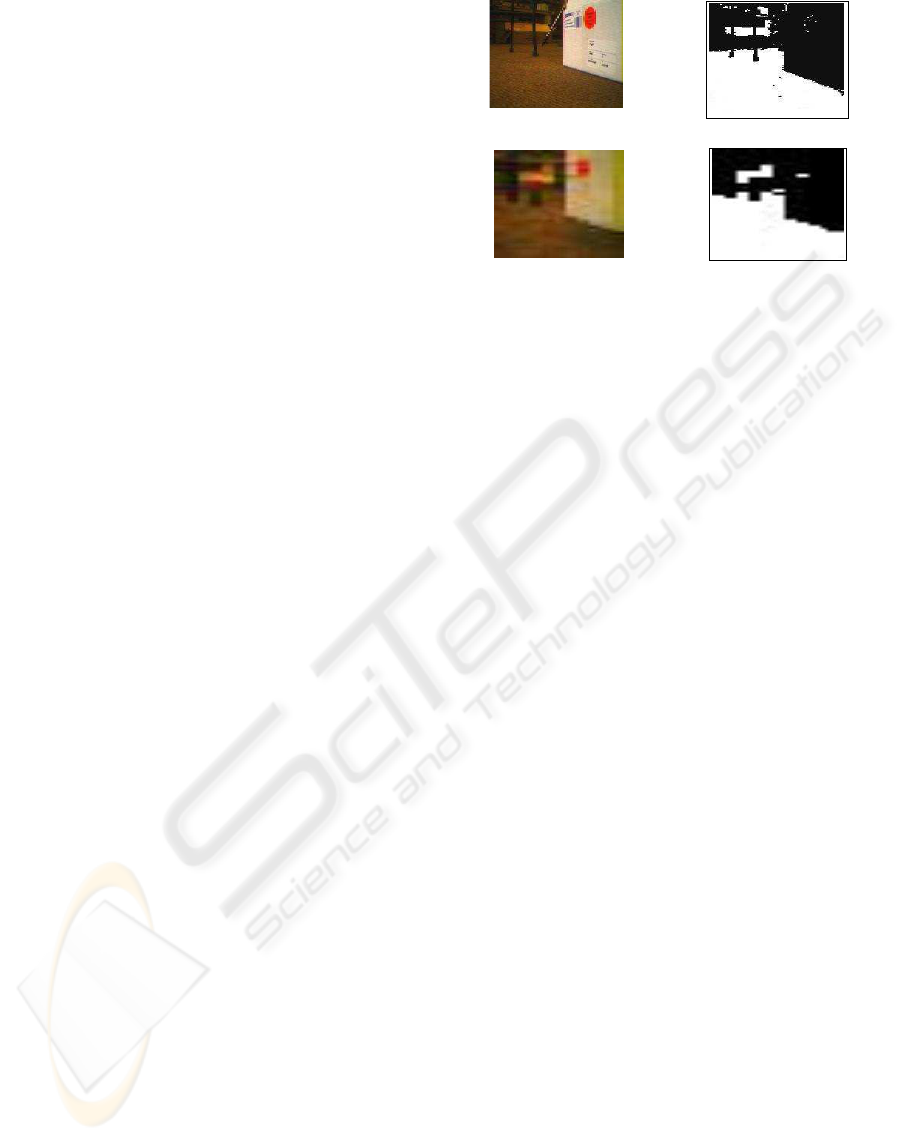
Figure 1: The images processed by the vision module. A
is a full resolution colour image. B is the binary obstacle-
ground image of A. C is a low resolution image from A and
D is its corresponding binary image.
the size of lookup table from 2
24
elements to 2
12
ele-
ments. Effectively, we make the classifier more gen-
eral since each element of the reduced table represents
a group of similar colours in the original space. We
also use very low resolution images of 22∗ 30 pixles.
Fig. 1 has two examples of the outputs from this seg-
mentation procedure. At the top row is a picture taken
from the camera mounted on our robot at the max-
imum resolution and the binary image produced by
the segmentation procedure. At the bottom row is the
down-sampling version of the top row picture and its
corresponding binary image.
The output of the image segmentation is a binary
image differentiating obstacles from the ground. As-
suming all objects have their bases on the ground,
the distance to an object is the distance to its base.
This distance is linear to the y-coordinate of the edge
between the object and the ground in the binary im-
age. For obstacle avoidance, we only need the dis-
tance and width of obstacles but not their height and
depth. Therefore a vector of distance measurements
to the nearest obstacles is sufficient, we call this ob-
stacle distance vector (ODV). We convert the binary
image to the required vector by copying the lowest y-
coordinate of a non-floor pixel in each column to the
corresponding cell in the vector. Each element of the
vector represents the distance to the nearest obstacle
in a specific direction.
2.2 Control Algorithm
The control algorithm we adopted is reactive, deci-
sions are made upon the most recent sensory readings.
The inputs to the controller are the obstacle distance
vector, produced by the visual module, and distance
measurements from the two sonar sensors pointing at
ICINCO 2007 - International Conference on Informatics in Control, Automation and Robotics
276
Procedure 1 PopulateLookupMap ( n: number of
pixels , P : array of n pixels.
for i = 0 to n− 1 do
(R,G,B) =⇐ rescale(P[i]
r
,P[i]
g
,P[i]
b
)
pixel counter[R][G][B] ⇐
pixel
counter[R][G][B] +1
end for
for (R,G,B) = (0,0,0) to MAX(R,G,B) do
is
ground map[R][G][B] ⇐
pixel
counter[R][G][B] > n∗ 5%
end for
return is
ground map
Procedure 2 is ground(p : pixel ).
(R,G,B) ⇐ rescale(p
r
, p
g
, p
b
)
return is
ground map[R][G][B];
the sides of the robot. The ODV gives a good resolu-
tion distance map of any obstacle in front of the robot.
Each cell in the vector is the distance to the nearest
obstacle in a direction of an angle of about 2.5
◦
. The
angular resolution of the two sonar sensors are much
lower. So the robot has a good resolution view at the
front and lower at the sides. The controlling mecha-
nism consists of several reflexive rules.
• If there are no obstacles detected in the area mon-
itored by the camera, run at maximum speed.
• If there are objects in front but further than a trig-
ger distance, slow down.
• If there are objects within the trigger distance,
start to turn to an open space.
• If a sonar sensor reports a veryclose object, within
5 cm, turn to the opposite direction.
The control algorithm does not calculate how far the
robot should turn. It will keep turning until the area
in front is clear. The robot looks for an open space
by first looking in the opposite direction to the per-
ceived obstacle, if the half image in that side is free
of obstacles, the robot will turn to this direction. If
there are obstacles in both left and right half of the
image, the two measurements from sonar sensors are
compared and the robot will turn to the direction of
the sonar sensor that reports no existence of obstacles
or a biger distance measurement. There is no attempt
to incorporate or fuse data from the camera and sonar
sensors together into a uniformed representation. The
algorithm uses the sensor readings as they are.
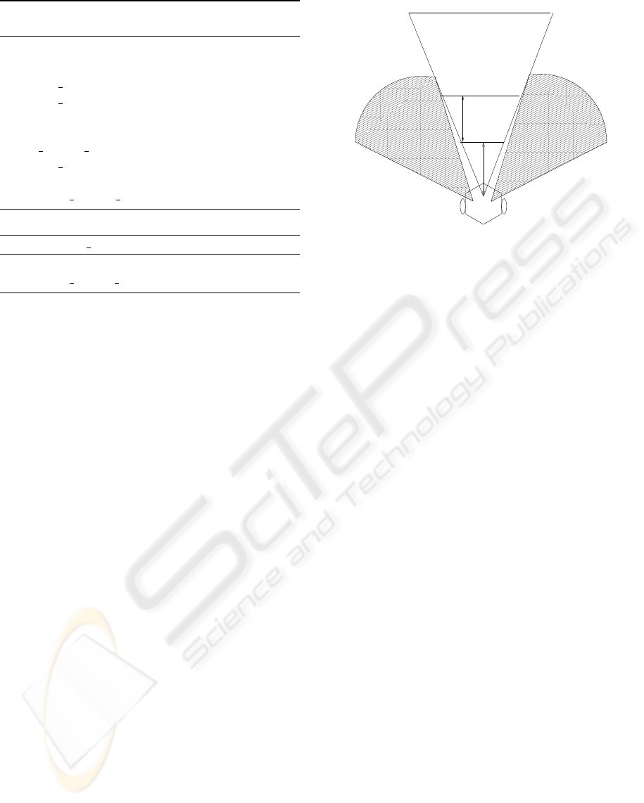
15cm
15cm
A
B
D C
E F
Figure 2: A visualisation of the monitored area. ABCD :
the area captured by the camera. Shaded areas represent
the sonar sensors views. Segment EF is the trigger distance
line.
3 PLATFORM CONFIGURATION
AND IMPLEMENTATION
The robot control software runs on a Gumstix (gum,
), a small Linux computer that has an Intel 200 MHz
ARM processor with 64 Mb of RAM. The vision sen-
sor is a CMUcam2 module connected to the Gumstix
via a RS232 link. A Brainstem micro-controller is
used to control sonar sensors and servos. The robot
is driven by two servos. These electronic devices are
mounted on a small three wheeled robot chassis. The
total cost of all the components is less than 300 US
dollars. The robot can turn on the spot with a small
radius of about 5 cm. Its maximum speed is 15cm/s.
The robot is powered by 12 AA batteries. A fully
charged set of batteries can last for up to 4 hours.
Fig. 2 shows the area in front of the robot that is
monitored by the robot’s sensors. The CMUcam is
mounted on the robot pointing forward at horizontal
level,15 cm above the ground, and captures an area of
about 75cm
2
. Because the camera has a relatively nar-
row FOV of about 55
◦
, the two sonar sensors on the
side are needed. In total, the robot’s angle of view is
120
◦
. The robots dimensions are 20cm∗ 20cm∗ 15cm.
The hardware configuration was determined by the
trial and error method. The parameters we presented
here were the best that we found and were used in the
experiments reported in section IV.
The maximum frame resolution of the CMUCam2
is 87 ∗ 144 pixels, we lower the resolution to only
22 ∗ 30 pixels. We only need the first bottom half
of the picture so the final image has dimensions of
22∗ 15. In our implementation, the obstacle distance
vector has 22 cells, each cell corresponds to an angle
VISION-BASED OBSTACLE AVOIDANCE FOR A SMALL, LOW-COST ROBOT
277
of 2.5
◦
. The vector is then outputted to the controller.
Since the control algorithm doesn’t build a model,
there is no need to convert the pixel’s y-coordinates
to an absolute measurement e.g. cm or inch. Because
the resolution of the images is very low, the distance
estimation is not very accurate. At the lowest row of
the image, where the ratio between pixel and the pro-
jected real world area is highest, each pixel represents
an area of 2∗ 1.5cm
2
.
The distance that triggers the robot to turn is set
to 30 cm. The robot needs to turn fast enough so that
an obstacle will not be closer than 15 cm in front of it
since the distance of any object in this area can not be
calculated correctly. At maximum speed , the robot
will have about two seconds to react and if the robot
has already slowed down while approaching the ob-
ject, it will have about three seconds. We have tried
different combinations of trigger distances and turn-
ing speeds to achieve a desirable combination. The
first criteria is that the robot must travel safely, this
criteria sets the minimum turning speed and distance.
The width of view of the camera at the distance of
30 cm from the robot or 35 cm from the camera is
30 cm. The width of our robot is 20 cm, so if the vi-
sion module does not find an obstacle inside the trig-
ger range, the robot can safely move forward. The
second criteria is the robot needs to be able to go
to cluttered areas. This means it should not turn too
early when approaching objects. Also when the robot
is confronted by the wall or a large object, it should
turn just enough to move along the wall/object and
not bounce back. This criteria encourages the robot
to explore the environment.
4 EXPERIMENTS
4.1 Experiment Setup and Results
We tested the robot in two environments, a 1.5∗ 2.5m
2
artificial arena surrounded by 30cm height walls and
an office at the University of Kent Computing de-
partment, shown in Fig. 3. The surface of the arti-
ficial arena is a flat cartoon board with green wall-
papers on top. We put different real objects such as
boxes, shoes, books onto the arena. We first tested the
robot in the arena with no objects (the only obstacless
are walls) and then made the tests more difficult by
adding objects. The office is covered with a carpet.
The arena presents a more controlable environment
where the surface is smooth and relatively colour-
uniformed. The office environmnent is more chal-
lenging where even though the ground is flat its sur-
face is much more coarse and not colour-uniformed.
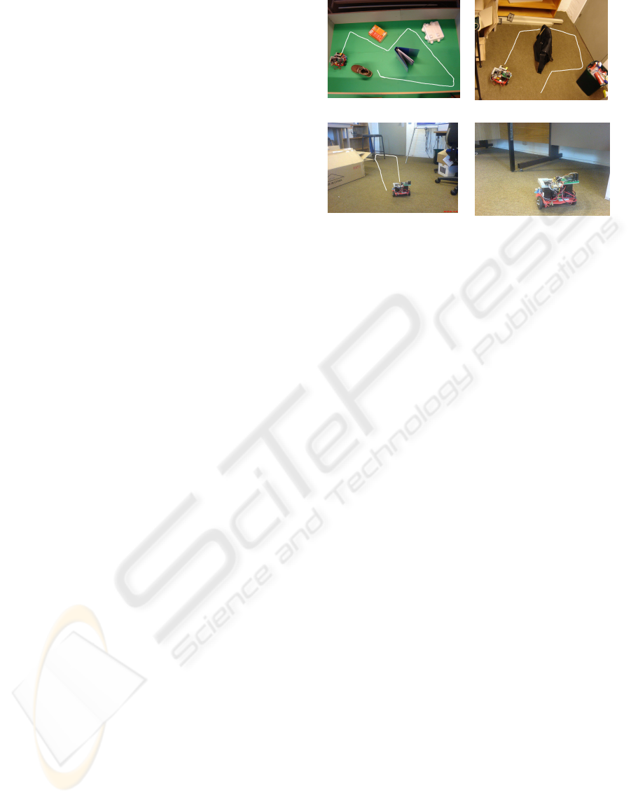
A B
C
D
Figure 3: Snapshots of the robot in the test environments
and its trajectories. A: the artificial arena with 4 objects.
B: A small area near the office corner. C: A path that went
through a chair’s legs. D: An object with no base on the
ground.
For each test, the robot run for 5 mins. We placed
the robot in different places and put different objects
into the test area. In general, the robot is quite compe-
tent; Table I summaries the result. The vision-based
obstacle detection module correctly identified obsta-
cle with almost 100% accuracy, that is if there was an
obstacle in the camera view, the algorithm would reg-
ister an non-ground area. Although the calculated dis-
tances of obstacles are not very accurate, they provide
enough information for the controller to react. The
simple mechanism of finding an open space worked
surprisingly well. The robot was good at finding a
way out in a small area such as the areas under tables
and between chairs. The number of false positives are
also low and only occured in the office environment.
This is because the office’s floor colours are more dif-
ficult to capture thoroughly. Further analysis revealed
that false positives often occurred in the top part of the
images. This is explained by the ratio of pixels/area
in the upper part of the image being lower than the
bottom part. At the top row of the image, each pixel
corresponds to an area of 7 ∗ 4cm while at the bot-
tom row the area is 2∗ 1.5cm. Fortunately, the upper
part also corresponds to the further area in real world.
Therefore, most false positive cases resulted in unnec-
essary decreasing of speed but not changing direction.
Because of the robot’s reactive behaviour, it is capable
of responding quickly to changes in the environments.
During some of the tests, we removed and put obsta-
cles in front of the robot. The robot could react to the
changes and altered it’s running direction accordingly.
Fig. 3 shows 4 snapshots of the robot during op-
eration and its trajectory. In picture A, the robot ran
in the arena with 4 obstacles, it successfully avoided
ICINCO 2007 - International Conference on Informatics in Control, Automation and Robotics
278
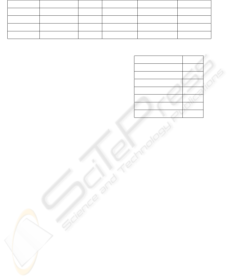
Table 1: Performance summary.
Environment No of Obstacles Duration Average speed No. of collisions False positive
Arena 0 60 min 13 cm/c 0 0%
Arena 1 60 min 10 cm/s 0 0%
Arena 4 60 min 6 cm/s 2 0%
Office > 10 180 min 9 cm/s 7 3%
all the objects. On picture B, the robot went into a
small area near a corner with a couple of obstacles
and found a way out. On picture C, the robot success-
fully navigated through a chair’s legs which presented
a difficult situation. Picture D was a case where the
robot failed to avoid an obstacle. Because the table
leg cross-bar is off the floor, the robot underestimated
the distance to the bar.
4.2 Discussion
We found that adding more obstacles onto the arena
did not increase the number of collisions significantly.
However the average speed of the robot dropped as
the arena became more crowded. The speed loss is
admitedly due to the robot’s reactive behaviour. The
robot does not do path planning therefore it can not
always select the best path. In some cluttered areas,
the robot spent a lot of time spinning around before it
could find a viable path. We can improve the robot’s
behaviour in these situations by having a mechanism
to detect cluttered and closed areas so the robot can
avoid them.
Each control cycle takes about 150ms or 7Hz. Ta-
ble II shows the time spent on each task in the cycle.
The algorithm used only 15% of the CPU during op-
eration. This leaves plenty of resources for higher be-
haviours if needed. It is possible to implement this al-
gorithm with a less powerful CPU. Since only 10% of
the CPU time is spent on processing data, a CPU run-
ning at 20 MHz would be sufficient. So instead of the
Gumstix computer we can use a micro-controller such
as a Brainstem or a BASIC STAMP for both image
processing and motion control without any loss in per-
formance. The memory usage is nearly one Mb which
is rather big. We did not try to optimise memory us-
age during implementation so improvements could be
made. We plan to implement this control algorithm
on a micro-controller instead of the Gumstix. This
change will reduce the cost and power usage of the
robot by a large amount. To the best of our knowl-
edge, there has not been a mobile robot that can per-
form reliable obstacle avoidance in unconstrained en-
vironments using such low resolution vision and slow
microprocessor.
Table 2: Speed performance.
Task Time
Image acquiring 95 ms
Sonar sensor reading 125 ms
Image processing 5 ms
Controller 1 ms
Servos updating < 1ms
Logging 3 ms
Total 150 ms
REFERENCES
http://www.gumstix.org.
Braitenberg, V. (1984). Vehicles: Experiments in Synthetic
Psychology. MIT Press/Bradford books.
Brooks, R. A. (1985). A robust layered control system for a
mobile robot. Technical report, MIT, Cambridge, MA,
USA.
Lenser, S. and Veloso, M. (2003). Visual sonar: fast ob-
stacle avoidance using monocular vision. In Intelli-
gent Robots and Systems, 2003. (IROS 2003). Pro-
ceedings. 2003 IEEE/RSJ International Conference
on, volume 1, pages 886–891.
Lorigo, L., Brooks, R., and Grimsou, W. (1997). Visually-
guided obstacle avoidance in unstructured environ-
ments. In Intelligent Robots and Systems, 1997. IROS
’97., Proceedings of the 1997 IEEE/RSJ International
Conference on, volume 1, pages 373–379, Grenoble,
France.
Ulrich, I. and Nourbakhsh, I. R. (2000). Appearance-based
obstacle detection with monocular color vision. In
AAAI/IAAI, pages 866–871.
VISION-BASED OBSTACLE AVOIDANCE FOR A SMALL, LOW-COST ROBOT
279
