
FAST ESTIMATION FOR RANGE IDENTIFICATION IN THE
PRESENCE OF UNKNOWN MOTION PARAMETERS
Lili Ma, Chengyu Cao, Naira Hovakimyan, Craig Woolsey
Department of Aerospace and Ocean Engineering, Virginia Tech, Blacksburg, VA 24061-0203
Warren E. Dixon
Department of Mechanical and Aerospace Engineering, University of Florida, Gainesville, FL 32611-6250
Keywords:
Fast adaptive estimator, Range identification.
Abstract:
A fast adaptive estimator is applied to the problem of range identification in the presence of unknown mo-
tion parameters. Assuming a rigid-body motion with unknown constant rotational parameters but known
translational parameters, extraction of the unknown rotational parameters is achieved by recursive least square
method. Simulations demonstrate the superior performance of fast estimation in comparison to identifier based
observers.
1 INTRODUCTION
A variety of 3D motion estimation algorithms have
been developed since 1970’s, inspired by such dis-
parate applications as robot navigation, medical imag-
ing, and video conferencing. Even though motion es-
timation from imagery is not a new topic, continual
improvements in digital imaging, computer process-
ing capabilities, and nonlinear estimation theory have
helped to keep the topic current. Assuming that the
motion of the moving object follows certain structure,
which can have parametric uncertainties, extended
Kalman filter (EKF) has been used to estimate the
states and parameters of the nonlinear system asso-
ciated with the moving object dynamics. Application
of EKF assumes linearization about the estimated tra-
jectory. However, for the motion estimation from im-
agery the geometric structure of the perspective sys-
tem can be lost during the linearization
(Ghosh et al.,
1994; Dixon et al., 2003). Refs. (Jankovic and Ghosh,
1995; Chen and Kano, 2002; Dixon et al., 2003; Kara-
giannis and Astolfi, 2005; Ma et al., 2005) have con-
sidered nonlinear observers for perspective dynamic
systems (PDS) arising in visual tracking problems. In
general, a PDS is a linear system, whose output is
observed up to a homogeneous line(Chen and Kano,
2
002). This class of nonlinear observers is referred to
as perspective nonlinear observers.
Perspective nonlinear observers (Jankovic and
Ghosh, 1995; Chen and Kano, 2002; Dixon et al.,
2003; Karagiannis and Astolfi, 2005; Ma et al.,
2005) are used quite often for determining the un-
k
nown states (i.e., the 3D Euclidean coordinates) of
a moving object with known motion parameters. For
example, an identifier-based observer was proposed
in(Jankovic and Ghosh, 1995) to estimate a station-
ary point’s 3D position using a moving camera. An-
other discontinuous observer, motivated by sliding
mode and adaptive methods, is developed in(Chen
and Kano, 2002) that renders the state observation
error uniformly ultimately bounded. A state esti-
mation algorithm with a single homogeneous obser-
vation (i.e., a single image coordinate) is presented
in(Ma et al., 2005). A reduced-order nonlinear ob-
server is described in(Karagiannis and Astolfi, 2005)
to provide asymptotic range estimation. All these re-
sults are based on the assumption that the object is
following a known motion dynamics in the 3D space.
In this paper, we discuss a situation when some
of the motion parameters, more specifically, the rota-
tional parameters, are unknown constants. The objec-
tive is to achieve fast state estimation and parameter
convergence.
One model for the relative motion of a point in
the camera’s field of view is the following linear
system
(Jankovic and Ghosh, 1995; Chen and Kano,
2
002; Dixon et al., 2003; Karagiannis and Astolfi,
157
Ma L., Cao C., Hovakimyan N., Woolsey C. and E. Dixon W. (2007).
FAST ESTIMATION FOR RANGE IDENTIFICATION IN THE PRESENCE OF UNKNOWN MOTION PARAMETERS.
In Proceedings of the Four th International Conference on Informatics in Control, Automation and Robotics, pages 157-164
DOI: 10.5220/0001642001570164
Copyright
c
SciTePress

2005):
˙
X(t)
˙
Y(t)
˙
Z(t)
=
0 w
1
w
2
−w
1
0 w
3
−w
2
−w
3
0
X(t)
Y(t)
Z(t)
+
b
1
b
2
b
3
,
(1)
where the matrix [w
i
] presents the rotational dynam-
ics, the vector [b
i
] corresponds to the translational mo-
tion, while [X, Y, Z]
⊤
are the coordinates of the point
in the camera frame. From the 2D image plane, the
homogeneous output observations are given by
x
1
(t) = X(t)/Z(t), x
2
(t) = Y(t)/Z(t). (2)
These equations might model either a stationary
point’s 3D position as observed from a moving cam-
era (assuming that the moving camera’s velocities can
be measured
(Jankovic and Ghosh, 1995)) or a mov-
ing point’s 3D position as observed from a stationary
camera(Tsai and Huang, 1981). In general, w
i
can be
time-dependent, but in this paper we limit the discus-
sion to constant w
i
’s.
Let
x(t) = [x
1
(t), x
2
(t), x
3
(t)]
⊤
= [X(t)/Z(t), Y(t)/Z(t), 1/Z(t)]
⊤
.
(3)
The system (1) with output observations (3) is equiv-
alent to the system
˙x
1
(t)
˙x
2
(t)
=
b
1
−b
3
x
1
b
2
−b
3
x
2
x
3
+
w
2
+ w
1
x
2
+ w
2
x
2
1
+ w
3
x
1
x
2
w
3
−w
1
x
1
+ w
2
x
1
x
2
+ w
3
x
2
2
,
˙x
3
(t) = (w
2
x
1
+ w
3
x
2
)x
3
−b
3
x
2
3
,
(4)
with the output
y(t) = [x
1
(t),x
2
(t)]
⊤
. (5)
Estimation of x
3
(t) from the measurements
(x
1
(t),x
2
(t)) constitutes the range identification
problem. Refs.
(Jankovic and Ghosh, 1995; Chen
and Kano, 2002; Dixon et al., 2003; Karagiannis and
Astolfi, 2005; Ma et al., 2005) have solved this prob-
lem assuming that the motion parameters w
i
and b
i
in
(1) are known (where i ∈ {1,2, 3}). Here, we assume
that the parameters w
i
are unknown. The objective,
then, is to estimate x
3
(t) as well as the unknown
parameters w
i
. This problem can be formulated in a
way such that an existing i
dentifier-based observer
(IBO), described in
(Jankovic and Ghosh, 1995),
can be applied, such that under certain assumptions,
the approach provides exponential convergence of
both the range and the parameter estimates. A more
general case of the problem is discussed in
(Ma et al.,
2007)
, where the rotational matrix is represented by a
3×3 matrix instead of the skew-symmetric matrix as
in (1).
In this paper, a recently-developed novel adaptive
estimator is applied for the estimation of x
3
(t) along
with the unknown parameters w
i
. A numerical com-
parison of the performance of this adaptive estimator
with the IBO observer is provided.
The paper is organized as follows. Range identi-
fication in the presence of unknown parameters via
the IBO is presented in Sec. 2. A brief review of
the fast estimator is given in Sec. 3. In Sec. 4, fast
estimation for the range identification problem with
unknown motion parameters is presented. Section 5
presents the simulation results. Section 6 extends the
analysis to general affine motion. Finally, section 7
concludes the paper.
2 RANGE IDENTIFICATION IN
THE PRESENCE OF UNKNOWN
PARAMETERS VIA IBO
Consider the state estimation problem for the perspec-
tive dynamic system (7), where the motion parameters
w
i
(for i = 1,2, 3) are assumed to be unknown con-
stants. Let θ be a vector of these unknown constants
defined as
θ = [w
1
, w
2
, w
3
]
⊤
. (6)
The system (4) can be rewritten as
˙x
1
(t)
˙x
2
(t)
= w
⊤
s
(x
1
,x
2
)
x
3
θ
, (7a)
˙x
3
(t)
˙
θ
=
(w
2
x
1
+ w
3
x
2
)x
3
−b
3
x
2
3
|
{z }
g
s
(x
1
,x
2
,x
3
,w
2
,w
3
)
0
3×1
, (7b)
with
w
⊤
s
(x
1
,x
2
) =
b
1
−b
3
x
1
x
2
1+ x
2
1
x
1
x
2
b
2
−b
3
x
2
−x
1
x
1
x
2
1+ x
2
2
,
(8)
which fits into the form of the general nonlinear sys-
tem to which IBO might be applicable, by regarding
x
1
= [x
1
,x
2
]
⊤
, x
2
= [x
3
,θ
⊤
]
⊤
, and φ(x
1
,u) = 0 (please
refer to
(Jankovic and Ghosh, 1995) for details of the
IBO).
To apply the IBO observer, we need the following
assumption for the system in (7):
Assumption 2.1
1. Let x(t) =
x
1
(t),x
2
(t),x
3
(t),θ
⊤
⊤
be bounded
kx(t)k< M, M > 0 for every t ≥ 0. Let Ω = {x ∈
R
n
: kx(t)k < M}. Further, for some fixed con-
stant γ > 1, let Ω
γ
= {x ∈ R
n
: kx(t)k< γM}.
2. The function w
s
(x
1
,x
2
) and its first time deriva-
tive are piecewise smooth and uniformly bounded.
ICINCO 2007 - International Conference on Informatics in Control, Automation and Robotics
158

Suppose that there exist positive constants L
1
,L
2
such that
kw
⊤
s
(x
1
,x
2
)k < L
1
,
dw
⊤
s
(x
1
,x
2
)
dt
< L
2
. (9)
Further, there do not exist constants κ
i
(for i =
1,2, 3,4) with
∑
4
i=1
κ
2
i
6= 0 such that
κ
1
v
1
(τ)+ κ
2
v
2
(τ)+ κ
3
v
3
(τ)+ κ
4
v
4
(τ) = 0, (10)
for all τ ∈ [t,t + µ], where µ > 0 is a sufficiently
small constant, and v
i
(τ) denotes the i
th
column
in w
s
in (8).
It is straightforward to verify that, under Assump-
tion 2.1, the system in (7) verifies the assumptions re-
quired for the application of IBO. Estimation of x
3
(t),
along with the unknown motion parameters θ, can be
obtained via direct application of the IBO, as given
below.
Letting e
1
= ˆx
1
−x
1
, e
2
= ˆx
2
−x
2
, e
3
= ˆx
3
−x
3
, the
following observer can be designed for the system (7)
˙
ˆx
1
˙
ˆx
2
= GA
e
1
e
2
+ w
⊤
s
(x
1
,x
2
)
ˆx
3
ˆ
θ
,
˙
ˆx
3
˙
ˆ
θ
= −G
2
w
s
(x
1
,x
2
)P
e
1
e
2
+
g
s
(x
1
,x
2
, ˆx
3
, ˆw
2
, ˆw
3
)
0
3×1
,
ˆ
x(t
+
i
) = M
ˆ
x(t
−
i
)
k
ˆ
x(t
−
i
)k
,
(11)
where x denotes [x
1
,x
2
,x
3
,θ
⊤
]
⊤
,
ˆ
θ denotes the esti-
mation of θ, and the sequence of t
i
is defined as
t
i
= min {t : t > t
i−1
andk
ˆ
x(t)k≥ γM}, t
0
= 0, (12)
for some fixed constant γ > 1. The closed-loop error
dynamics can be derived from (7) and (11) as
˙e
1
˙e
2
= GA
e
1
e
2
+ w
⊤
s
(x
1
,x
2
)
e
3
˜
θ
,
"
˙e
3
˙
˜
θ
#
= −G
2
w
s
(x
1
,x
2
)P
e
1
e
2
+
g
s
(x
1
,x
2
, ˆx
3
, ˆw
2
, ˆw
3
) −g
s
(x
1
,x
2
,x
3
,w
2
,w
3
)
0
3×1
,
(13)
where
˜
θ =
ˆ
θ−θ and
˙
˜
θ =
˙
ˆ
θ, since θ is assumed to be
a constant vector. The main claim is that there ex-
ists a positive constant G
0
, such that the estimation
errors [e
1
,e
2
,e
3
,
˜
θ
⊤
]
⊤
converge to zero exponentially
if the constant G in (11) is chosen to be larger than
G
0
(Jankovic and Ghosh, 1995).
3 FAST ESTIMATOR
Range identification in the presence of unknown mo-
tion parameters is further pursued using a recently-
developed fast adaptive estimator. The adaptive es-
timator enables estimation of the unknown time-
varying parameters in the system dynamics via fast
adaptation (large adaptive gain) and a low-pass filter.
If the time-varying unknown signal is linearly param-
eterized in unknown constant parameters, the adap-
tive estimator can be further augmented by a recur-
sive least-square algorithm (RLS) to estimate the un-
known constant parameters asymptotically
(Cao and
Hovakimyan, 2007)
.
In the following, main results of the the adaptive
estimator are given for the purpose of completeness.
More details are presented in
(Cao and Hovakimyan,
2007)
.
3.1 Preliminaries
Some basic definitions from linear system theory are
given in this section.
Definition 3.1 For a signal ξ(t), t ≥ 0, ξ ∈ R
n
, its
L
∞
norm is defined as
kξk
L
∞
= max
i=1,...,n
sup
τ≥0
|ξ
i
(τ)|
, (14)
where ξ
i
is the i
th
component of ξ.
Definition 3.2 The
L
1
gain of a stable proper single–
input single–output system H(s) is defined as:
kHk
L
1
=
∞
0
|h(t)|dt, (15)
where h(t) is the impulse response of H(s).
Definition 3.3 For a stable proper m input n output
system H(s) its
L
1
gain is defined as
kHk
L
1
= max
i=1,...,n
m
∑
j=1
kH
ij
k
L
1
!
, (16)
where H
ij
(s) is the i
th
row j
th
column element of H(s).
3.2 Problem Formulation
Consider the following system dynamics:
˙x(t) = A
m
x(t) + ω(t), x(0) = x
0
, (17)
where x ∈ R
n
is the system state vector (measurable),
ω(t) ∈ R
n
is a vector of unknown time-varying sig-
nals or parameters, and A
m
is a known n×n Hurwitz
matrix. Let
ω(t) ∈ Ω, (18)
where Ω is a known compact set. The signal ω(t) is
further assumed to be continuously differentiable with
uniformly bounded derivative
k
˙
ω(t)k≤ d
ω
< ∞, ∀ t ≥ 0, (19)
where d
ω
can be arbitrarily large. The estimation ob-
jective is to design an adaptive estimator that provides
fast estimation of ω(t).
FAST ESTIMATION FOR RANGE IDENTIFICATION IN THE PRESENCE OF UNKNOWN MOTION
PARAMETERS
159

3.3 Fast Adaptive Estimator
The adaptive estimator consists of the state predictor,
the adaptive law and a low-pass filter, which extracts
the estimation information.
State Predictor: We consider the following state
predictor:
˙
ˆx(t) = A
m
ˆx(t) +
ˆ
ω(t), ˆx(0) = x
0
, (20)
which has the same structure as the system in (17).
The only difference is that the unknown parameters
ω(t) are replaced by their adaptive estimates
ˆ
ω(t) that
are governed by the following adaptation laws.
Adaptive Laws: Adaptive estimates are given by:
˙
ˆ
ω(t) = Γ
c
Proj(
ˆ
ω(t),−P˜x(t)),
ˆ
ω(0) =
ˆ
ω
0
, (21)
where ˜x(t) = ˆx(t)−x(t) is the error signal between the
state of the system and the state predictor, Γ
c
∈ R
+
is
the adaptation rate, chosen sufficiently large, and P is
the solution of the algebraic equation A
⊤
m
P + PA
m
=
−Q, Q > 0.
Estimation: The estimation of the unknown sig-
nal is generated by:
ω
e
(s) = C(s)
ˆ
ω(s), (22)
where C(s) is a diagonal matrix with its i
th
diagonal
element C
i
(s) being a strictly proper stable transfer
function with low-pass gain C
i
(0) = 1. One simple
choice is
C
i
(s) =
θ
a
s+ θ
a
. (23)
3.4 Convergence Results
The fast adaptive estimator in Sec. 3.3 ensures that
ω
e
(t) estimates the unknown signal ω(t) with the final
precision:
k1−C(s)k
L
1
kωk
L
∞
+
γ
c
√
Γ
c
, (24)
where k·k
L
1
denotes the
L
1
gain of the system.
To quantify this performance bound between
ω
e
(t) and ω(t), an intermediate signal ω
r
(t) is intro-
duced as:
ω
r
(s) = C(s)ω(s). (25)
The following theorem gives the performance
bound between ω
e
(t) and ω
r
(t). Details of the proof
can be found in
(Cao and Hovakimyan, 2007).
Theorem 3.1 For the system in (17) and the fast
adaptive estimator in (20), (21) and (22), we have
kω
e
−ω
r
k
L
∞
≤
γ
c
√
Γ
c
, (26)
where
γ
c
= kC(s)H
−1
(s)k
L
1
r
ω
m
λ
min
(P)
, (27a)
H(s) = (sI −A
m
)
−1
, (27b)
ω
m
= max
ω∈Ω
4kωk
2
+ 2
λ
max
(P)
λ
min
(Q)
d
ω
max
ω∈Ω
kωk
, (27c)
and k·k
L
∞
denotes the
L
∞
norm of the signal.
Corollary 3.1 For the system in (17) and the fast
adaptive estimator in (20), (21) and (22), we have
lim
Γ
c
→∞
(ω
e
(t) −ω
r
(t)) = 0, ∀ t ≥ 0. (28)
We further characterize the performance bound
between ω
r
(t) and ω(t). For simplicity, we use a first
order C(s) as in (23). It follows from (25) that
˙
ω
r
(t) = −θ
a
ω
r
(t) + θ
a
ω(t), ω
r
(0) = 0. (29)
We note that ω
r
(t) can be decomposed into two com-
ponents:
ω
r
(t) = ω
r
1
(t) + ω
r
2
(t), (30)
where ω
r
1
(t) and ω
r
2
(t) are defined via:
˙
ω
r
1
(t) = −θ
a
ω
r
1
(t)+ θ
a
ω(t), ω
r
1
(0) = ω(0),(31a)
˙
ω
r
2
(t) = −θ
a
ω
r
2
(t), ω
r
2
(0) = −ω(0). (31b)
It follows from (31a) that
kω
r
1
−ωk
L
∞
= k1−C(s)k
L
1
kωk
L
∞
. (32)
Since
lim
θ
a
→∞
k1−C(s)k
L
1
= 0, (33)
the norm kω
r
1
− ωk
L
∞
can be rendered arbitrarily
small by increasing the bandwidth of C(s). Further,
ω
r
2
(t) decays to zero exponentially and the settling
time is inverse proportional to the bandwidth of C(s).
Increasing the bandwidth of C(s) implies that ω
r
2
(t)
decays to zero quickly.
From (26) and (32), when the transients of C(s)
due to the initial condition −ω(0) die out, ω
e
(t) es-
timates ω(t) with the final precision given in (24).
It is obvious that both the final estimation precision
and the transient time can be arbitrarily reduced by
increasing the bandwidth of C(s), which leads to
smaller
L
1
gain for k1−C(s)k
L
1
. However, the large
bandwidth of C(s) leads to further increase of γ
c
,
which requires large Γ
c
to keep the term
γ
c
√
Γ
c
small.
We note that larger Γ
c
implies faster computation and
requires smaller integration step.
3.5 Extraction of Unknown Parameters
If the time-varying signal ω(t) can be linearly param-
eterized in unknown constant parameters and known
ICINCO 2007 - International Conference on Informatics in Control, Automation and Robotics
160

nonlinear functions, extraction of the unknown pa-
rameters can be achieved by recursive least-square
(RLS) algorithm under certain persistent excitation
type of condition. The RLS algorithm is reviewed be-
low.
Consider a linear scalar regression model denoted
as:
ω
k
= θ
⊤
φ
k
+ e
k
, (34)
where
θ = [θ
1
,θ
2
,··· ,θ
n
]
⊤
(35)
is the n×1 vector of the plant parameters, and
φ
k
= [φ
k,1
,φ
k,2
,··· ,φ
k,n
]
⊤
(36)
is the n ×1 regressor vector at time instant k, while
e
k
is a zero-mean discrete white noise sequence with
variance σ
2
k
. When the observation of (ω
k
,φ
k
) has
been obtained for k = 1, ··· ,N (with N > n), the RLS
estimate for θ, denoted by
ˆ
θ, can be obtained in the
following discrete form
(Verhaegen, 1989):
L
k
=
P
k−1
φ
k
λ+ φ
⊤
k
P
k−1
φ
k
,
ˆ
θ
k
=
ˆ
θ
k−1
+ L
k
(ω
k
−φ
⊤
k
ˆ
θ
k−1
),
P
k
=
1
λ
P
k−1
−
P
k−1
φ
k
φ
⊤
k
P
k−1
λ+ φ
⊤
k
P
k−1
φ
k
!
,
(37)
where P
0
= pI
p×p
and λ ∈ (0,1]. Coefficients p and λ
are design gains and need to be chosen appropriately.
When φ
k
is persistently exciting during the observa-
tion period, RLS algorithm ensures the convergence
of
ˆ
θ to θ. The convergence rate of RLS can be in-
creased by choosing large λ.
The PE condition of the regressor vector is defined
as
(Verhaegen, 1989):
Definition 3.4 The regressor vector φ
k
is persistently
exciting over the observation interval k
0
≤ k ≤ k
N
with an exponentially forgetting factor λ ≤ 1, if the
following condition is fulfilled:
αI ≤
k
N
∑
k=k
0
φ
k
φ
⊤
k
λ
k
N
−k
≤ βI (38)
for some positive α > 0 and β > 0.
4 FAST ESTIMATION FOR
RANGE IDENTIFICATION IN
THE PRESENCE OF
UNKNOWN PARAMETERS
Denote
η(t) =
η
1
(t)
η
2
(t)
, (39)
and write equation (7a) as
˙x
1
(t)
˙x
2
(t)
= w
⊤
s
(x
1
,x
2
)
x
3
(t)
θ
= η(t). (40)
From equations (6), (8), and (40), we have
b
1
−b
3
x
1
x
2
1+ x
2
1
x
1
x
2
b
2
−b
3
x
2
−x
1
x
1
x
2
1+ x
2
2
x
3
(t)
w
1
w
2
w
3
= η(t).
(41)
Multiplying the first equation in (41) by T
2
= b
2
−
b
3
x
2
(t) and subtracting the second equation from it
pre-multiplying it by T
1
= b
1
−b
3
x
1
(t), we arrive at:
T
2
x
2
+ T
1
x
1
,T
2
(1+ x
2
1
) −T
1
x
1
x
2
,T
2
x
1
x
2
−T
1
(1+ x
2
2
)
|
{z }
φ
⊤
(t)
w
1
w
2
w
3
|
{z}
θ(t)
= [T
2
η
1
−T
1
η
2
].
(42)
Recursive least squares method can be used to extract
w
i
’s according to (37), with ω replaced by T
2
η
1
−
T
1
η
2
. Once w
i
(for i = 1, 2,3) are available, equation
(41) takes the form:
b
1
−b
3
x
1
b
2
−b
3
x
2
x
3
=
η
1
η
2
−
x
2
1+ x
2
1
x
1
x
2
−x
1
x
1
x
2
1+ x
2
2
w
1
w
2
w
3
,
(43)
where x
3
(t) can be extracted using pseudo-inverse.
Using the fast adaptive estimator described in
Sec. 3, estimation of η(t), denoted by η
e
(t), can be
obtained via the following steps:
• State Estimator:
˙
ˆx
1
˙
ˆx
2
= A
m
˜x
1
˜x
2
+
ˆ
η(t),
˜x
1
˜x
2
=
ˆx
1
−x
1
ˆx
2
−x
2
. (44)
• Adaptive Law (use large Γ
c
):
˙
ˆ
η(t) = −Γ
c
P
⊤
˜x
1
˜x
2
⊤
. (45)
• Extraction:
η
e
(s) = C(s)
ˆ
η(s), C(s) =
C
s+C
. (46)
According to Corollary 3.1, the final estimation pre-
cision η
e
(t) −η(t) and the transient time to achieve
this can be arbitrarily reduced by increasing the band-
width of C(s). Increasing the bandwidth of C(s) re-
quires larger Γ
c
.
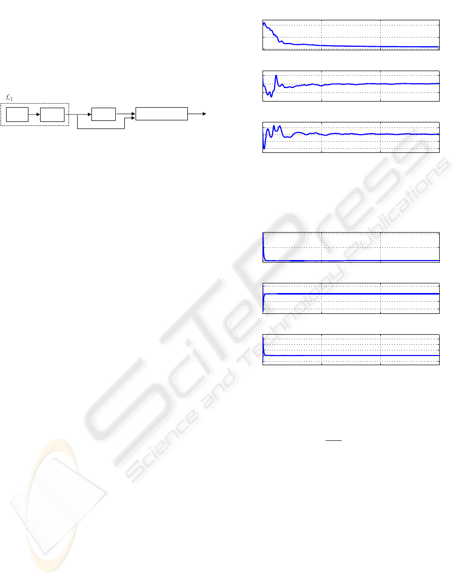
The flow chart of state and parameter estimation
of a rigid motion using the fast adaptive estimator is
illustrated in Fig. 1. In the first step of estimating η(t),
both the estimation precision and transient time can
be arbitrarily reduced by increasing the bandwidth of
C(s) and using larger Γ
c
. In the second step of extract-
ing ˆw
i
’s from η
e
(t) using the recursive least square
FAST ESTIMATION FOR RANGE IDENTIFICATION IN THE PRESENCE OF UNKNOWN MOTION
PARAMETERS
161
method, fast speed can be achieved by properly tun-
ing the RLS gains. Estimation of x
3
(t), denoted by
ˆx
3
(t), can be obtained from η
e
(t) and ˆw
i
’s via pseudo-
inverse. Since the fast adaptive estimator assumes
minimization of the
L
1
gain of 1 −C(s) for perfor-
mance improvement, it is referred to as
L
1
adaptive
estimator.
)(t
e
η
)(
ˆ
3
tx
)(
ˆ
t
η
)(sC
Adaptive Estimator
RLS
)(
ˆ
tw
i
Pseudo-inverse
Figure 1: Flow chart of L
1
adaptive estimator.
5 SIMULATION RESULTS
State estimation of [x
3
(t),θ
⊤
]
⊤
using the IBO ob-
server (11) and the fast adaptive estimator (44) (46)
are implemented in Matlab, where the motion dynam-
ics are selected to be
˙
X(t)
˙
Y(t)
˙
Z(t)
=
0 −4 −0.8
4 0 −0.6
0.8 0.6 0
X(t)
Y(t)
Z(t)
+
10
3πsin(2πt)
3πsin(2πt +π/4)
,
(X
0
,Y
0
,Z
0
) = (1,1.5,2.5), x
0
= (X
0
/Z
0
,Y
0
/Z
0
,1/Z
0
).
(47)
First, we present simulation results in the ideal case
with no measurement noise. The parameters for the
IBO observer and the fast adaptive estimator are cho-
sen to be:
• IBO (referring to (11)):
G = 10, ( ˆx
3
(0), ˆw
1
(0), ˆw
2
(0), ˆw
3
(0)) = (0,0,0,0).
• Fast adaptive estimator (referring to (37), (45),
(46)):
p = 100, λ = 0.99999, A
m
= −I
2
,
(
ˆ
η
1
(0),
ˆ
η
2
(0)) = (0,0), Γ
c
= 2×10
8
, C = 200.
In both cases, we set ( ˆx
1
(0), ˆx
2
(0)) =
(x
1
(0),x
2
(0)), M = 30, A = I
2
, P = −1/2 × I
2
,
where I
2
denotes the 2×2 identity matrix.
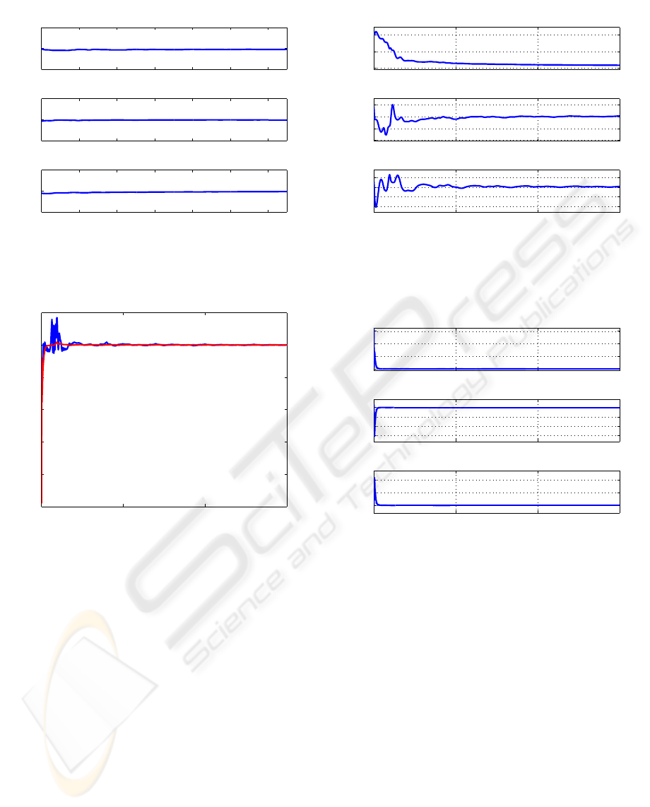
Estimation of w
i
(for i = 1,2, 3) with the use of the
IBO and the fast adaptive estimator is shown in Fig-
ures 2 and 3, respectively. Figure 4 shows the zoomed
version of Figure 3 for the steady state error. State es-
timation error of x
3
is plotted in Figure 5 for compar-
ison of both methods.
From Figures 2 and 3, it can be observed that the
fast adaptive estimator achieves faster estimation of
the motion parameters. The same is true for x
3
.
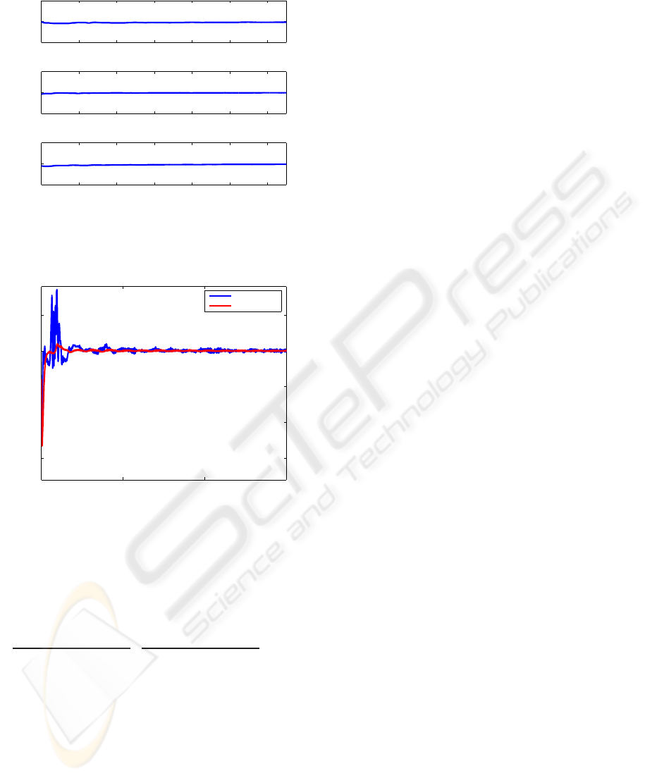
Simulation results are also presented in Figs. 6∼9
when the output is noise-corrupted with uniform
bound ±10
−2
. The simulation parameters are the
same as above. In this case, when extracting ˆx
3
(t), the
output from the pseudo-inverse is further processed
0 5 10 15
0
2
4
Estimation of w
1
− w
1
0 5 10 15
−2
−1
0
1
Estimation of w
2
− w
2
0 5 10 15
−2
−1
0
1
Estimation of w
3
− w
3
Figure 2: Estimation of motion parameters using IBO
(without measurement noise).
0 5 10 15
0
50
100
Estimator of w
1
− w
1
0 5 10 15
−40
−20
0
20
Estimator of w
2
− w
2
0 5 10 15
−10
0
10
20
30
Estimator of w
3
− w
3
Figure 3: Estimation of motion parameters using fast adap-
tive estimator (without measurement noise).
using a low-pass filter
30
s+30
to give the final state esti-
mation. We observe that corresponding plots with or
without measurement noise are very similar.
6 FURTHER EXTENSION
In this paper, rigid-body motion is considered that
contains only three rotational parameters (w
1
,w
2
,w
3
)
as given in (1). For general affine motion described
by
˙
X(t)
˙
Y(t)
˙
Z(t)
=
a
11
a
12
a
13
a
21
a
22
a
23
a
31
a
32
a
33
X(t)
Y(t)
Z(t)
+
b
1
b
2
b
3
, (48)
the rotational matrix contains nine parameters. As-
suming that the [a
ij
] (for i, j = 1, 2,3) are unknown
ICINCO 2007 - International Conference on Informatics in Control, Automation and Robotics
162
2 4 6 8 10 12 14
−0.5
0
0.5
Estimator of w
1
− w
1
2 4 6 8 10 12 14
−0.5
0
0.5
Estimator of w
2
− w
2
2 4 6 8 10 12 14
−0.5
0
0.5
Estimator of w
3
− w
3
Figure 4: Enlarged view of Fig. 3 (without measurement
noise).
0 5 10 15
−5
−4
−3
−2
−1
0
1
Figure 5: Comparison of state estimation errors (without
measurement noise).
constants, the method described in Sec. 4 cannot lead
to extraction of the nine unknown parameters in a
straightforward way.
The system (48) with output observations (3) is
equivalent to the system
˙x
1
(t)
˙x
2
(t)
=
b
1
−b
3
x
1
b
2
−b
3
x
2
x
3
+
a
13
+ (a
11
−a
33
)x
1
a
23
+ a
21
x
1
+
a
12
x
2
−a
31
x
2
1
− a
32
x
1
x
2
(a
22
−a
33
)x
2
−a
31
x
1
x
2
− a
32
x
2
2
,
˙x
3
(t) = −(a
31
x
1
+ a
32
x
2
+ a
33
)x
3
−b
3
x
2
3
,
(49)
with the output (5). The above system can also be
rewritten in the form of (7a), where θ and w
⊤
s
(x
1
,x
2
)
take the forms
θ = [a
11
, a
12
, a
13
, a
21
, a
22
, a
23
, a
31
, a
32
, a
33
]
⊤
,
(50)
0 5 10 15
0
2
4
Estimation of w
1
− w
1
0 5 10 15
−2
−1
0
1
Estimation of w
2
− w
2
0 5 10 15
−2
−1
0
1
Estimation of w
3
− w
3
Figure 6: Estimation of motion parameters using IBO (with
measurement noise).
0 5 10 15
0
50
100
150
Estimator of w
1
− w
1
0 5 10 15
−30
−20
−10
0
Estimator of w
2
− w
2
0 5 10 15
0
10
20
Estimator of w
3
− w
3
Figure 7: Estimation of motion parameters using fast adap-
tive estimator (with measurement noise).
and
w
⊤
s
(x
1
,x
2
) =
b
1
−b
3
x
1
x
1
x
2
1 0 0 0
b
2
−b
3
x
2
0 0 0 x
1
x
2
1
−x
2
1
−x
1
x
2
−x
1
−x
1
x
2
−x
2
2
−x
2
,
(51)
respectively. Following the logic in Sec. 4, we can
write the following system of algebraic equations
w
⊤
s
(x
1
,x
2
)
x
3
a
11
a
12
··· a
33
⊤
=
η
1
η
2
,
(52)
with the w
⊤
s
(x
1
,x
2
) given in (51). Again, multiplying
the first equation in (52) by T
2
= b
2
−b
3
x
2
and sub-
tracting the second equation from it pre-multiplying it
FAST ESTIMATION FOR RANGE IDENTIFICATION IN THE PRESENCE OF UNKNOWN MOTION
PARAMETERS
163
2 4 6 8 10 12 14
−0.5
0
0.5
Estimator of w
1
− w
1
2 4 6 8 10 12 14
−0.5
0
0.5
Estimator of w
2
− w
2
2 4 6 8 10 12 14
−0.5
0
0.5
Estimator of w
3
− w
3
Figure 8: Enlarged view of Fig. 7 (with measurement
noise).
0 5 10 15
−1.5
−1
−0.5
0
0.5
estimation error of x
3
IBO
fast estimator
Figure 9: Comparison of state estimation errors (with mea-
surement noise).
by T
1
= b
1
−b
3
x
1
, we arrive at:
[T
2
(x
1
,x
2
,1), T
1
(x
1
,x
2
,1), (b
1
x
2
−b
2
x
1
)(x
1
,x
2
,1)]
|
{z }
φ
affine
(t)
a
11
a
12
.
.
.
a
33
= [T
2
η
1
−T
1
η
2
].
(53)
The nine columns in φ
affine
(t) in (53) are linearly de-
pendent. It is obvious that the 7
th
,8
th
, and 9
th
columns
can be presented as linear combinations of the first
six columns. For example, column
9
can be written
as column
9
= column
5
−column
1
. Thus, extraction
of the nine unknown parameters cannot be performed
by the recursive least square method since it violates
the PE condition in (38). Further research will ex-
plore the use of adaptive observers for general affine
motion identification.
7 CONCLUSION
A recently developed fast adaptive estimator is ap-
plied to the range identification problem of a rigid
motion in the presence of unknown motion parame-
ters. Fast convergence speed is achieved compared to
existing nonlinear perspective observers.
ACKNOWLEDGEMENTS
This work was sponsored in part by ONR Grant
#N00014-06-1-0801 and AFOSR MURI subcontract
F49620-03-1-0401.
REFERENCES
Cao, C. and Hovakimyan, N. (2007). Fast adaptive estima-
tor for time-varying unknown parameters. To Appear
in American Control Conference.
Chen, X. and Kano, H. (2002). A new state observer for per-
spective systems. IEEE Trans. on Automatic Control,
47(4):658–663.
Dixon, W., Fang, Y., Dawson, D., and Flynn, T. (2003).
Range identification for perspective vision systems.
IEEE Trans. on Automatic Control, 48(12):2232–
2238.
Ghosh, B., Jankovic, M., and Wu, Y. (1994). Perspective
problems in system theory and its application to ma-
chine vision. Journal of Mathematical Systems, Esti-
mation and Control, 4(1):3–38.
Jankovic, M. and Ghosh, B. (1995). Visually guided rang-
ing from observations of points, lines and curves via
an identifier based nonlinear observer. Systems and
Control Letters, 25:63–73.
Karagiannis, D. and Astolfi, A. (2005). A new solution
to the problem of range identification in perspective
vision systems. IEEE Trans. on Automatic Control,
50(12):2074–2077.
Ma, L., Cao, C., Hovakimyan, N., Dixon, W., and Woolsey,
C. (2007). Range identification in the presence of un-
known motion parameters for perspective vision sys-
tems. To Appear in American Control Conference.
Ma, L., Chen, Y., and Moore, K. (2005). Range identifica-
tion for perspective dynamic system with a single ho-
mogeneous observation. International Journal of Ap-
plied Mathematics and Computer Science, 15(1):63–
72.
Tsai, R. and Huang, T. (1981). Estimating three-
dimensional motion parameters of a rigid planar
patch. IEEE Trans. on Acoustic, Speech, and Signal
Processing, ASSP-29(6):1147–1152.
Verhaegen, M. H. (1989). Round-off error propagation in
four generally-applicable, recursive, least-squares es-
timation schemes. Automatica, 25(3):437–444.
ICINCO 2007 - International Conference on Informatics in Control, Automation and Robotics
164
