ELECTRO HYDRAULIC PRE-ACTUATOR MODELLING OF AN
HYDRAULIC JACK
Salazar Garcia Mahuampy, Viot Philippe
Laboratoire Matériaux Endommagement Fiabilité et Ingénierie des Procédés (LAMEFIP), France
Nouillant Michel
Keywords: Three-stage servo-valve, modeling, hydraulic jack.
Abstract: Before the realization of testing devices such as a high speed (5m/s) hydraulic hexapod with a high load
capacity (60 tons and 6 tons for static and dynamic operating mode), the simulation is an essential step.
Hence from softwares such as SimMecanics, we have performed an electro hydraulic model of the servo-
valve-jack part by using parameters and recorded results with mono axis testing bench of high-speed
hydraulic jack (5m/s), which has a high loading capacity (10 tons for static and 1 ton for dynamic operating
mode). The high-speed jack is provided by two parallel three-stage servo-valves. Each three-stage servo-
valve supplies 600L/mm. Therefore the unit allows us to obtain a realistic model of an extrapolated hexapod
from the mono axis currently used. The aim of this article is to provide a modeling of the second and third
stage servo valves by comparison of the typical experimental reading and the computed curves obtained
from simulation.
1 INTRODUCTION
The main difficulties of the modeling of an actuator
hydraulic hexapod are servo valve models. In the
case of electrical actuators operating in control
voltage, the torque is got from the control voltage
and the rotation speed of the motor. In the case of
hydraulic actuator, for a current control of servo
valve given, the efforts provided by the jack depend
on the flow rate and consequently they depend also
on the speed of the jack and leakages. This aspect is
not taken into account by using the classical
frequency model of the servo valve (Faisandier,
1999), (Mare, 2002), (Thayer, 1965).
At first, we will present the hydraulic model of
the servo valve + jack system. In a second time, a
nonlinear modeling will be developed. Lastly, the
results obtained from the modeling will be presented
and analyzed.
2 ELECTRO HYDRAULIC
SYSTEM
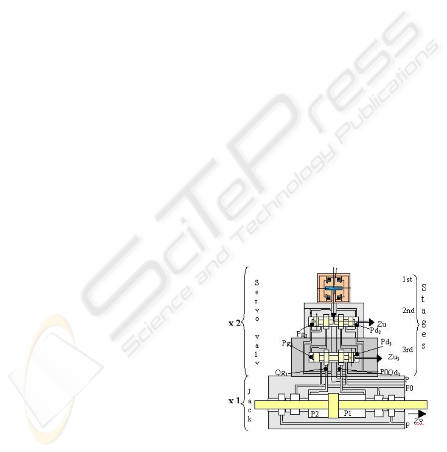
Figure 1: Diagrammatic section of system.
Figure 1 shows a model with three-stage servo valve
and a jack. The symbol "x2" and "x1" indicate
respectively the presence in the system of two
59
Garcia Mahuampy S., Philippe V. and Michel N. (2007).
ELECTRO HYDRAULIC PRE-ACTUATOR MODELLING OF AN HYDRAULIC JACK.
In Proceedings of the Fourth International Conference on Informatics in Control, Automation and Robotics, pages 59-64
DOI: 10.5220/0001632900590064
Copyright
c
SciTePress
parallel servo valves supplying the jack. A servo
valve is controlled by an electrical stage (1
st
stage),
followed by a 2nd stage and a 3rd hydraulic
amplification stage (Faisandier,1999), (Guillon,
1961).
A control current applied to the system input is
named i. The double potentiometric hydraulic
divisor of the first stage, leads to two pressures Pg
2
and Pd
2
applied to the end of the slide on the 2nd
stage, the flow rates provided by this 2nd stage are
named Qg
2
and Qd
2
, applied to the control of the
slide displacement of the 3rd stage of the servo
valve.
The third stage generates the flow rates Qg
3
and
Qd
3
taking part in the sum of the flows entering and
going out of the jack chambers, and leading, through
instantaneous volumes of the chambers, and the
compressibility coefficient of the oil, to the pressure
variation in each chamber. The servo valve is
supplied with pressure P
0
and reservoir return line P.
3 MODELING
3.1 Servo Valve Linear Model
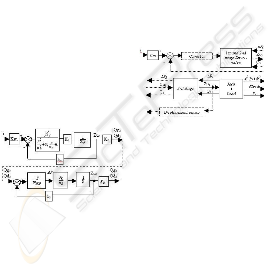
Figure 2 shows linear diagram of a servo valve
modeling (Pommier,2000).
Figure 2: Linear diagram of the servo valve.
Km: Gain between the current and the torque.
ωn: Undamped natural frequency of the pallet inertia of
the 1st stage.
ξ : Damping ratio of the friction of the pallet.
kf: Gain displacement in torque of the nozzle pallet unit.
K
1
: Gain in flow rate of hydraulic amplification.
S
2
: Surface of the slide ends of the 2nd stage.
k
w
: Gain of the feedback torque.
K’
2
: Gain in flow rate of the 2nd stage slide.
V
03
: Effective volume when the slide is centered.
S
3
: Surface of the slide ends of the 3rd stage.
m
3
: Slide mass of the 3rd stage.
K’
3
: Gain in flow rate of the 3rd stage.
One notes that for this model, the K’
2
and K’
3
coefficients characterize the flow rate as a function
of the slide positions. For the second stage, the K’
2
coefficient gives a good approximation within a
large part of the operating area, contrary to the K’3
coefficient suggesting that the speed of the jack does
not depend on the load.
3.2 Hydraulic Nonlinear Model
Figure 3 shows the general diagram describing the
non-linear model of servo-valve-jack system.
Figure 3: Nonlinear model of the servo valve + jack.
One takes into account the hydrodynamic forces
applied to the various slides of the servo valves.
These forces take part in the nonlinear behavior of
the device. This functional diagram shows that the
behavior of the servo valve and the jack cannot be
dissociated and must be treated as such.
We have developed a nonlinear model of the
servo-valve-jack unit allowing to determine, for a
given control current, the effort supplied by the jack
from the pressure variations within the control
volumes formed by the jack chambers. This pressure
variation after temporal integration defines the
pressure within the right and left chambers of the
jack. The difference of these pressures multiplied by
the active section of the piston gives the effort
supplied by the jack.
In our case, the main difficulty is the nonlinear
modeling of the servo valve; more particularly we
have to take into account a finite number of sensitive
parameters and the hydraulic nonlinear behavior
laws. In addition to the nonlinearities resulting from
the hydraulic potentiometer, the pressure flow will
be taken into account from the following relation:
ICINCO 2007 - International Conference on Informatics in Control, Automation and Robotics
60
.|P|K=Q Δ (1)
We assume that the flow rate of the fluid is
viscous and incompressible, as turbulent type.
The transient flow rate associated with fluid
incompressibility is proportional to the rate of
change of pressure in a volume of control and may
be expressed as:
se QQdtdVdtdPV −=+ )/()/)(/(
β
(2)
Where β is the bulk modulus of the fluid.
We also take into account the hydrodynamic
forces on the various slides of the servo-valves,
leading to the nonlinear behavior of the device.
(
)
gQF
hd
/2
γ
=
(3)
Where γ is the specific gravity (kg/m3) and g is
the gravitational acceleration.
The angular displacement of the frame engine
versus the current is given by:
)(
.
2
2
...
222
θθθϕθ
signFLKrJLZuKrPliKm ss +++=−Δ+
(4)
With ∆P2=Pg2-Pd2 difference of pressure
between the two slide ends of the 2nd stage.From
the equation (2) one can obtain the evolution laws of
the pressures Pg2 and Pd2.
⎟
⎠
⎞
⎜
⎝
⎛
−−+−
+
=
.
222021
2202
2
ZuSPgPKfQQg
ZuSVdt
dPg
b
β
⎟
⎠
⎞
⎜
⎝
⎛
+−+−
−
=
.
222021
2202
2
ZuSPdPKfQQd
ZuSVdt
dPd
b
β
(5)
(6)
Where, S
2
Z
u2
is the flow rate caused by the
motion of the slide and Qg
1
and Qd
1
are the flow
rates resulted from the pressure applied to the
section of fixed openings S1, Qb is the flow rate
from the nozzle tip.
By applying the fundamental principle of
dynamics we obtain the sum of the forces applied to
the slide of the 2nd stage:
)(
.
22
.
22
..
222222
θψθ
signFZuKrZuZumFLKrPS shd +++=−−Δ
(7)
Where S2ΔP2 is the difference of forces applied
to the ends of the slide, Kr2Lθ is the force due to the
stiffness and the deformation of the pallet.
The flow rate Qd2 and Qg2 provided by the 2nd
stage is given by the equation (1). The equation of
Qd2, Qg2 taking into account the slide covering and
the resulting leakage. The modeling of the slide
covering is exponential modeling, where ε is a
constant. The very low value of ε ensures the
continuity in the opening model of the slide and the
leakage resulted from the slide covering.
From the equation (2), and (7), one can obtain
the evolution laws of the pressures and the sum of
the forces related to the third stage and the jack
hydraulic.
4 IMPLEMENTATION AND
RESULTS
At first, we have identified the parameters of the
nonlinear model from the high-speed 5m/s servo-
valve-jack unit of LAMEFIP laboratory. This first
step gives us some experimental reference
parameters for the validity of our servo-valve model.
The servo valve composed of the first and second
stages and the second servo valve composed of the
third stage are respectively hydaustar 550 and 1160
type servo valve. All the parameter values of the
model estimated or measured of the electro
hydraulic system for the second and third stages are
summarized in table 1.
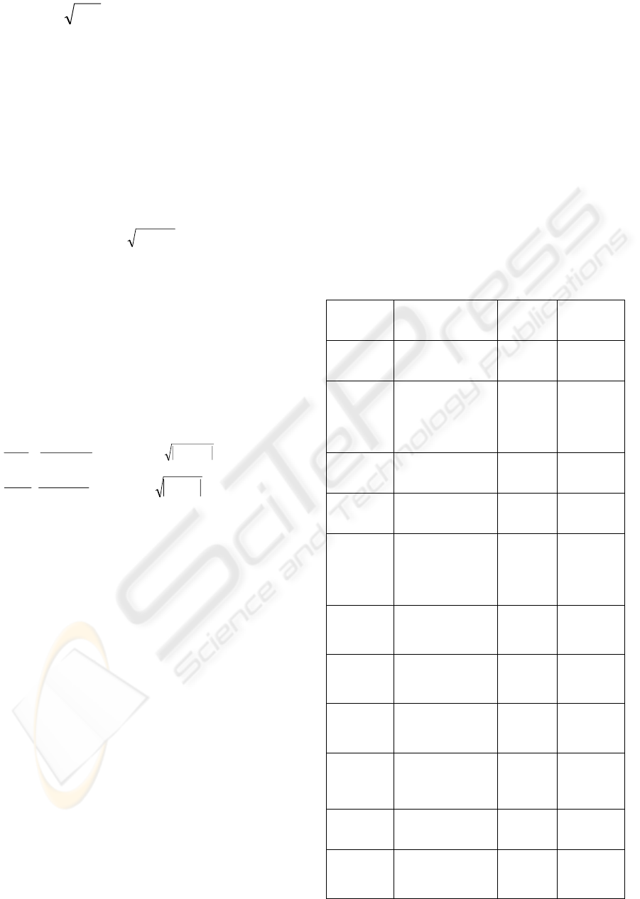
Table 1: Parameter values of the second and third stages.
Parameters
Manufact
urer data
Estimated
data
L
Length magnetic
pallet
31.2e-3
(m)
-----------
l
Outdistance
between magnetic
axis pallets and
metering jets
10.5e-3
(m)
------------
Dbuse
Diameter of nozzle
tip
0.18e-3
(m)
----------
Sbuse
Surface of nozzle
tip
2.54e-8
(m
2
)
xo
Length between
magnetic axis
pallets and metering
jets
----------
55e-6
(m)
Kbuse Gain of nozzle tip ----------
0.039
(m
3
/s/m)
K1
Gain of flow rate of
the fixed section
----------
1.5e-9
(m
3
/s/m)
Kf
2
Gain of leakage in
the stage
----------
5.15e-12
(m
3
/s/m)
Vo
2
Volume control
when the slide is
centered
19.5e-9
(m
3
)
-----------
S
2
Surface of slide
3.38e-5
(m
2
)
-----------
J Pallet inertia ----------
4e-7
(Kg m
2
)
ELECTRO HYDRAULIC PRE-ACTUATOR MODELLING OF AN HYDRAULIC JACK
61
Φ
Viscous friction
coefficient in
rotation of the pallet
----------
9e-4
(Nm/rd s)
K
r2
Stiffness of the slide
of the stage
2100
(N/m)
------------
M
2
Slide masse 9e-3 (Kg) ------------
Ψ
2
Viscous friction
coefficient in slide
-------- 6 (Ns/m)
Kf
3
Gain of leakage in
the stage
-----------
1e-12
(m
3
/s/m)
Ε Lap ----------- 3.7e-6 (m)
K
2
Gain of flow rate of
volume control in
the stage
-----------
6e-4
(m
3
/s/m)
S
3
Surface of slide
5e-4 (m
2
)
------------
Vo
3
Volume control
when the slide is
centered
8.6e-6 (m
3
)
------------
M
3
Slide masse
276e-3
(Kg)
------------
Ψ
3
Viscous friction
coefficient in slide
-----------
1000
(Ns/m)
After completing the estimated parameters, we
compare the typical experimental datas supplied by
the manufacturer such as the flow rate – current
characteristics for the second stage, the frequency
response of the second and third stages with the
curves resulting from the model using both the
estimated values and the measured values.
4.1 Flow Rate – Current
Characteristics
We have compared the flow rate Qd2 of the second
stage of the servo valve under differential pressure
of 70 bar when the current i varies in the range [
-I
max
; +I
max
], I
max
is the maximum value of the
current modulus. The figure 4 shows the flow rate
Qd2 – current i characteristics for the 550
Hydraustar servo valve (second stage) supplied by
the manufacturer and those obtained from the model.
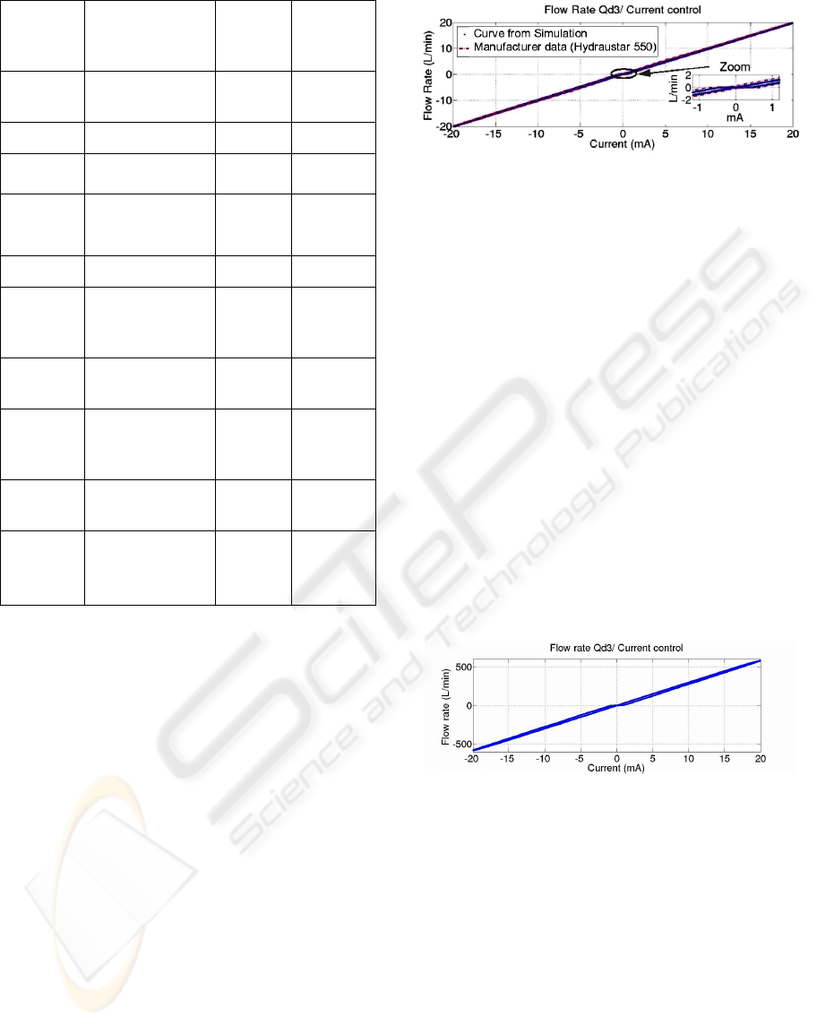
Figure 4: Flow rates / control currents characteristics
supplied by manufacturer and those obtained from the
model.
As shown in the figure 4, we can observe that the
result obtained from the model and that provided by
the manufacturer are similar when the current input
reaches the maximal value of 20 mA. The maximal
flow rate value provided by the driver servo valve
reaches 20 l/min. One can observe the role of the
leakages when the slide position is near the
hydraulic zero as shown in the inset of the figure4.
These leakages result from the taking into account of
the laps and the clearances between the slide and the
sleeve. The figure 5 shows the computed flow rate
Qd3 of the third stage of the servo valve under
differential pressure of 70 bar when the courant
varies from –I
max
and + I
max
. We obtain in this
particular configuration, a maximal computed value
of the flow rate provided by the servo valve of +/-
600 l/min. This value matches the manufacturer data
for this servo valve model.
Figure 5: Flow rate Qd3/ control current characteristics
obtained by simulation.
4.2 Frequency Response
We have compared the characteristic curves
obtained from the bench test measurement (by using
a servo valve flow with normalized decreasing of the
pressure of 70 bar for different input levels) with
the curves computed from our model.
4.2.1 First and Second Stage
The figure 6 shows the comparison of the
manufacturer curves with those obtained from the
model for the similar operating conditions: provided
ICINCO 2007 - International Conference on Informatics in Control, Automation and Robotics
62
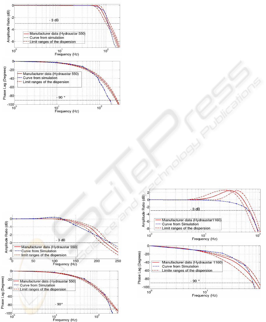
pressure Ps = 210 bar, differential pressure 70 bar,
100% nominal current.
Figure 6: Frequency response for 100% of the nominal
current. (for -3 dB, 110 Hz < f < 130 Hz, -90°, 230 Hz < f
< 250 Hz, theoretical curve).
The frequency response corresponding to 100 % of
nominal current obtained from the model gives a
cut-off frequency of 115 Hz for a gain of –3 dB and
a frequency of 180 Hz for a phase lag of 90°. The
cut-off frequency for –3 dB obtained with the model
is in the limit range of the dispersion of frequencies
provided by the manufacturer. For phase lag of 90°,
the frequency error between both curves is estimated
from 20% to 28 %.
Figure 7: Frequency response for 25 % of the nominal
current. (for –3 dB, 210 Hz < f < 230 Hz and for -90°, 250
Hz < f < 280 Hz, theoretical curve).
The figure 7 shows the frequency comparison of
the manufacturer curves and those obtained with the
model for the similar operating conditions: Provided
pressure Ps = 210 bar, pressure difference 70 bar,
25 % of the nominal current.
The frequency response for 25% of the nominal
current obtained from the model gives us a cut-off
frequency of 220 Hz for a gain of -3 dB and a
frequency of 210 Hz for a phase lag of 90°. The cut-
off frequency corresponding to a gain of -3 dB is in
the limit range of the dispersion of the manufacturer
frequencies. The frequencies related to the phase lag
of 90° obtained by modeling and those provided by
manufacturer are different. The error is estimated
from 16 % to 25 %. The computed curve shapes for
the second stage are different from those supplied by
the manufacturer. This difference should depend
directly on the estimated values of the pallet inertia
and its friction coefficient. An infinitesimal variation
of these values leads to the under damping observed
in amplitude plot of the bode diagram.
4.2.2 Third Stage
We compare the frequency responses of the serial
servo valve 1160, corresponding to the third stage,
with the coupling of the serial servo valve 550
related to the driving stage. The figure 8 shows the
typical response supplied by the manufacturer for
100 % of the nominal input signal.
Figure 8: Frequency response for 100 % of the nominal
current.
The driving servo valve is provided with a
pressure Ps of 210 bar. The cut-off frequencies in
the limit ranges of the dispersion for a frequency
response corresponding to 100 % of the nominal
ELECTRO HYDRAULIC PRE-ACTUATOR MODELLING OF AN HYDRAULIC JACK
63

current match respectively 70 Hz and 85 Hz for –3
dB and phase lag 90° for flow rates Qd3 and Qg3 of
600 l/min.
The frequency response for 100 % of the
nominal value of the current obtained from the
model gives a cut-off frequency of 70 Hz
corresponding to a gain of –3 dB and a frequency of
73 Hz for a phase lag of 90°. One observes that the
results obtained for the servo valves corresponding
to the second and third stages from the model and
those supplied by the manufacturer are close.
Nevertheless, one can note that a difference between
the curves amplitude from the manufacturer and
those obtained from the model. Indeed, the
manufacturer curves show an under damping
probably caused by the implementation of the
corrector in the system whereas we have performed
the modeling without corrections in loop control.
5 CONCLUSION
In our work, one can note that the servo valve is the
limiting element of the servo valve + jack system.
The flow rate values (20 l/min and 600 l/min
provided by the second and the third stage
respectively), like the bandwidth values of the
driving servo valve corresponding to the second
stage and those of the amplification stage e.g. the
third stage, obtained from the model and supplied by
manufacturer are rather similar. These results
suggest that the estimated values, which cannot be
measured, such as the gap xo between the nozzle and
the pallet, the inertia J and the viscous friction
coefficients of the pallet Φ, the friction coefficients
of the slides Ψ
2,
Ψ
3
and the flow rate gains Kbuse, K1,
Kf
2
, K2, Kf
3
, are fairly close to the physical values of
the type 550 and 1160 Hydraustar servo valve. We
have shown that the nonlinear model presented in
this work have allowed us the accurate simulation of
the nonlinear behavior of three stage servo valves
between the current input and the flow rate output.
This model allows the taking into account of the
pressure into the jack chambers as a function of the
forced stress. Hence with this model is possible to
computed the dynamic and static behavior, the latter
corresponds to the short circuit generated by jack
stoppers.
At this stage, the interfacing with the
SimMecanics software, by introducing as input this
corresponding to the effort between two ”bodies”,
the quantity (P1-P2)Sp (Sp: useful piston surface),
will provide as output from the software, the speed
and the relative position of both bodies.
ACKNOWLEDGEMENTS
Special thanks go to Mr. Terrade (Hydraustar
company) for supplying technical support.
REFERENCES
Faisandier, J., 1999. Mécanismes hydrauliques et
pneumatiques , 8
e
édition, Paris, Dunod.
Mare, J.C., 2002, Actionneurs Hydrauliques, Commande .
Techniques de l’ingénieurs, traité l’informatique
industrielle.S731.
Thayer, W.J., 1965, Transfer functions for moog servo
valves , Technical bulletin I03, MOOG INC. Springer-
Verlag.
Guillon, M., 1961, Etude et détermination des systèmes
hydrauliques, Paris, Dunod.
Pommier, V., Lanusse P., Oustaloup A., 2000, Commande
CRONE d'un actionneur hydraulique. In Journée
Franco-Tunisiennes, Monastir, Tunisie.
ICINCO 2007 - International Conference on Informatics in Control, Automation and Robotics
64
