
A DUAL MODE ADAPTIVE ROBUST CONTROLLER FOR
DIFFERENTIAL DRIVE TWO ACTUATED WHEELED MOBILE
ROBOT
Samaherni M. Dias, Aldayr D. Araujo
Department of Electrical Engineering, Federal University of Rio Grande do Norte, Brazil
Pablo J. Alsina
Department of Computer Engineering, Federal University of Rio Grande do Norte, Brazil
Keywords:
Variable Structure Systems, Adaptive Control, Decoupling, Nonholonomic Mobile Robot.
Abstract:
This paper is addressed to dynamic control problem of nonholonomic differential wheeled mobile robot. It
presents a dynamic controller to mobile robot, which requires only information of the robot configuration, that
are collected by an absolute positioning system. The control strategy developed uses a linear representation of
mobile robot dynamic model. This linear model is decoupled into two single-input single-output systems, one
to linear displacement and one to angle of robot. For each resulting system is designed a dual-mode adaptive
robust controller, which uses as inputs the reference signals calculated by a kinematic controller. Finally,
simulation results are included to illustrate the performance of the closed loop system.
1 INTRODUCTION
The control of mobile robot is a well known prob-
lem with nonholonomic constraints. There are many
works about it, and several of these works use kine-
matic model. Dynamic model, which is composed by
kinematic model plus the dynamic of robot, is used in
a few works.
An adaptive controller that compensates for cam-
era and mechanical uncertain parameters and ensures
global asymptotic position/orientation tracking was
presented by Dixon (Dixon et al., 2001). Chang
(Chang et al., 2004) proposes a novel way to de-
sign and analysis nonlinear controllers to deal with
the tracking problem of a wheeled mobile robots with
nonholonomic constraints.
The exact mobile robot model is complex and the
model has a lot of parameters to be considered, so
we will use a simplified model that consider some of
them. But this isn’t the only problem, because some
parameters can suffer variations, as the mass and the
frictional coefficients. For example, when robot is do-
ing a task as to carry an object, the object mass isn’t
considered by the model. So, we are using an associ-
ation between a dual mode adaptive robust controller
(DMARC) and a kinematic controller to the robot lin-
ear model.
The DMARC controller was presented in (Cunha
and Araujo, 2004) and it proposes a connection be-
tween a variable structure model reference adap-
tive controller (VS-MRAC, proposed by Hsu and
Costa(Hsu and Costa, 1989)) and a conventional
model reference adaptive controller (MRAC). The
goal is to have a robust system with fast response and
small oscillations (characteristics of VS-MRAC), and
a smooth steady-state control signal (characteristics
of the MRAC).
2 NONHOLONOMIC MOBILE
ROBOT
The robot considered in this paper is a nonholonomic
direct differential-drive two-actuated-wheeled mobile
robot, which is showed in Fig. 1. The robot is of
symmetric shape and the center of mass is at the geo-
metric center C of the body. It has two driving wheels
fixed to the axis that passes through C. Each wheel is
controlled by one independent motor.
Based on Fig 1, we have that d is distance between
wheels, r
d,e
are right and left wheels radius, ω
d,e
are
right and left wheels angle velocity, ω
r
is the angle
robot velocity, v
d,e
are right and left wheels linear ve-
39
M. Dias S., D. Araujo A. and J. Alsina P. (2007).
A DUAL MODE ADAPTIVE ROBUST CONTROLLER FOR DIFFERENTIAL DRIVE TWO ACTUATED WHEELED MOBILE ROBOT.
In Proceedings of the Fourth Inter national Conference on Informatics in Control, Automation and Robotics, pages 39-44
DOI: 10.5220/0001630900390044
Copyright
c
SciTePress
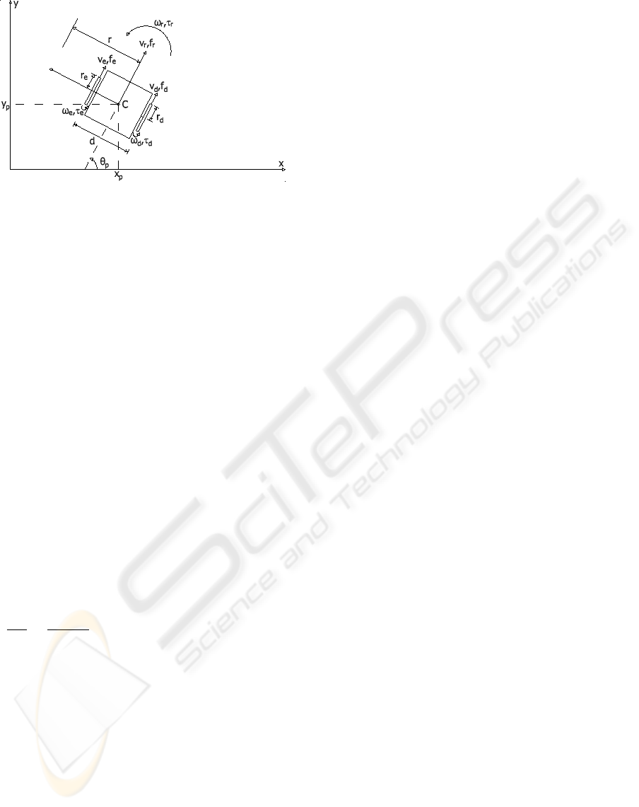
Figure 1: Differential-drive two-actuated-wheeled mobile
robot.
locity, v
r
is the linear robot velocity, τ
d,e
are right and
left wheels torque, τ
r
is the robot torque, f
d,e
are right
and left wheels force, f
r
is the robot force, θ
p
is the
angle of robot, x
p
is the x coordinate of C and y
p
is
the y coordinate of C.
2.1 Kinematic Model
The robot kinematic is described by equation (1),
˙q =
q
T
v
v (1)
q =
x
p
y
p
θ
p
q
T
v
=
cos(θ
p
) 0
sin(θ
p
) 0
0 1
v =
v
r
ω
r
The relation between velocity vectors (ω
at
and v)
is given by the equation ω
at
=
ω
T
v
v, with
ω
T
v
=
1/r
d
d/2r
d
1/r
e
−d/2r
e
ω
at
=
ω
d
ω
e
This mobile robot has a nonholonomic constraint,
because the driving wheels purely roll and don’t slip.
This constraint is described by
∂y
p
∂x
p
=
sin(θ
p
)
cos(θ
p
→ ˙y
p
cos(θ
p
) − ˙x
p
sin(θ
p
) = 0 (2)
2.2 Dynamic Model
The robot dynamic is represented by the following
equation
f = M
r
˙v + B
r
v (3)
which is composed by matrix M
r
and B
r
f =
f
r
τ
r
M
r
=
m 0
0 J
B
r
=
β
lin
0
0 β
ang
where β
lin
is the frictional coefficient to linear move-
ments, β
ang
is the frictional coefficient to angle move-
ments, m is the robot mass and J is the inertia mo-
ment.
It’s very important to consider the following rela-
tion
f =
ω
T
T
v
τ (4)
with τ is the vector
τ
d
τ
e
T
.
The DC motors dynamic is obtained of electrical
(5) and mechanical (6) equations,
i = R
m
e − R
m
K
m
ω
at
(5)
τ = K
m
i − J
m
˙
ω
at
− B
m
ω
at
(6)
where the vectors are
i =
i
d
i
e
R
m
=
1/R
d
0
0 1/R
e
e =
e
d
e
e
K
m
=
K
d
0
0 K
e
J
m
=
J
d
0
0 J
e
B
m
=
β
d
0
0 β
e
and e
d,e
are armature motor voltages, R
d,e
are wind-
ings resistances, K
d,e
are constants of induced volt-
age, J
d,e
are inertia moments of rotors, β
d,e
are mo-
tors frictional coefficients and i
d,e
are armature mo-
tors currents.
Using equation (5) in (6) and the result in (4), and
the force f , from (4), in equation (3), gives
K
v
= M
v
˙v + B
v
v (7)
where
K
v
=
ω
T
T
v
R
m
K
m
M
v
= M
r
+
ω
T
T
v
· J
m
·
ω
T
v
B
v
= B
r
+
ω
T
T
v
(R
m
K
2
m
+ B
m
)
ω
T
v
2.3 Linear Representation to Mobile
Robot Dynamic Model
A state-space model, with output vector Y = [S θ
p
]
T
,
is obtained from equation (7) and described by
˙x = Ax + Be
Y = Cx
(8)
where S is the linear displacement and
x =
v
r
ω
r
S
θ
p
A =
−M
−1
v
B
v
.
.
. 0
2×2
I
2×2
.
.
. 0
2×2
B =
M
−1
v
K
v
0
2×2
3 INVERSE SYSTEM
The right inverse system is used as an output con-
troller to force the original system output Y (t) to track
a given signal
U
S
U
θ
. The inverse system, in
this paper, is applied to decouple the original MIMO
ICINCO 2007 - International Conference on Informatics in Control, Automation and Robotics
40
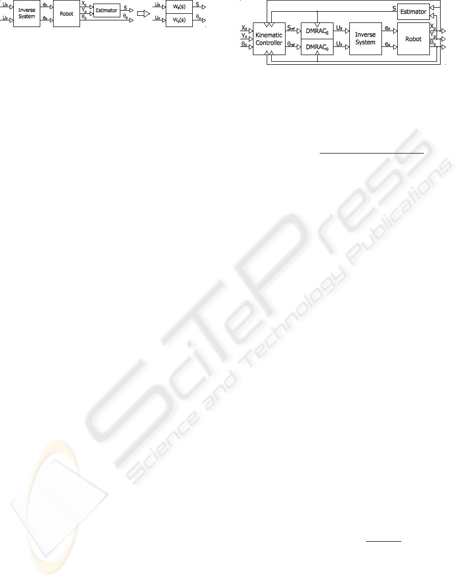
Figure 2: Decoupling based on an inverse system.
(Multiple-Input Multiple-Output) system (8) into two
SISO (Single-input Single-Output) systems (Fig. 2).
To get a stable inverse system, it’s necessary as-
sume that the system discussed is minimum phase.
The inversion algorithm of Hirschorn (Hirschorn,
1979) is applied to decouple the system (8). Deriving
the output vector Y =
S θ
p
T
two times the result-
ing system is
˙x = Ax + Be
¨
Y = C
2
x + D
2
e
(9)
where D
2
is an invertibility matrix, so the inverse sys-
tem is
˙
b
x =
b
A
b
x +
b
B
b
u
e =
b
Y =
b
C
b
x +
b
D
b
u
b
A = A − BD
−1
2
C
2
b
C = −D
−1
2
C
2
b
B = BD
−1
2
H
2
b
D = D
−1
2
H
2
b
u =
0 0 U
S
U
θ
T
H
2
= [0
2×2
I
2×2
]
The block diagram in Fig. 2 shows two indepen-
dent systems, which have the same transfer function
W
S
(s) = W
θ
(s) = 1/s
2
obtained by
W
S,θ
(s) = [C(sI − A)
−1
B] · [
b
C(sI −
b
A)
−1
b
B +
b
D]
where W
S,θ
(S) =
W
S
(s) W
θ
(s)
T
.
It’s important to remember that linear displace-
ment (S) is not measurable, so an estimated signal
is used. The linear model and the inverse system
need the exact robot parameters, and we are using
a simplified model with uncertain parameters. So a
robust adaptive controller will be used to guarantee
a good transient under unknown parameters and dis-
turbances. Two controllers are designed, one to each
transfer function.
4 CONTROLLER STRUCTURE
The controller structure is divided in five blocks (Fig.
3). First block, which is called kinematic controller,
it will calculate reference values (S
re f
and θ
re f
) based
on desired values (x
d
,y
d
,θ
d
) and absolute position-
ing system (x
p
,y
p
,θ
p
). Second block is composed by
two DMRAC controllers, which are projected to do
the robot to reach reference values. These controllers
based on references values will supply two control
signals (U
S
and U
θ
) to the inverse system. Third block
is the inverse system, fourth block is the robot and the
fifth block is the estimator.
Figure 3: Controller strategy block diagram.
4.1 Estimator
The linear displacement estimator is given by
S =
∑
i
sgn(X) ·
q
(x
i+1
− x
i
)
2
+ (y
i+1
− y
i
)
2
(10)
where X is
X = x
i+1
cos(θ
i
) +y
i+1
sin(θ
i
) −x
i
cos(θ
i
) −y
i
sin(θ
i
)
So, if X > 0, we have the linear displacement
(
c
4l > 0) and if X < 0, we have
c
4l < 0.
4.2 Kinematic Controller
The Fig 4 shows the new variables used in kinematic
controller as ∆l
pos
, that is the distance between robot
and any reference point (x
re f
,y
re f
), ∆λ
pos
is the dis-
tance of robot to point R
pos
that is nearest reference
point in robot orientation axis. φ
pos
is the angle of
robot orientation axis, (∆φ
pos
= φ
pos
− θ
p
). θ
d
is de-
sired orientation angle and γ is the difference between
φ and θ
d
angles (γ = φ − θ
d
).
To get that a robot leaves a point and reaches an-
other point it’s necessary ∆l
pos
→ 0 when t → ∞.
Based on decoupled linear model of robot a new
auxiliar point R
pos
(Fig 4) was proposed, to design
a positioning controller, because only in this point
∆λ
pos
= S
re f
− S. So, if ∆λ
pos
→ 0 and ∆φ
pos
→ 0,
the ∆l
pos
→ 0. The reference of DMARC
S
controller
is calculated by
S
re f
= ∆l
pos
· cos(∆φ
pos
) + S (11)
and the reference signal to DMARC
θ
controller is
given by
θ
re f
= φ
pos
= tan
−1
y
re f
− y
p
x
re f
− x
p
(12)
where the equations (11) and (12) represent the po-
sitioning controller and are using only informations
from absolute positioning system.
This work uses a mobile reference system to gen-
erate new points to the positioning controller for each
step of the algorithm. It’s based just in the robot kine-
matic model. The kinematic controller objective is to
A DUAL MODE ADAPTIVE ROBUST CONTROLLER FOR DIFFERENTIAL DRIVE TWO ACTUATED WHEELED
MOBILE ROBOT
41
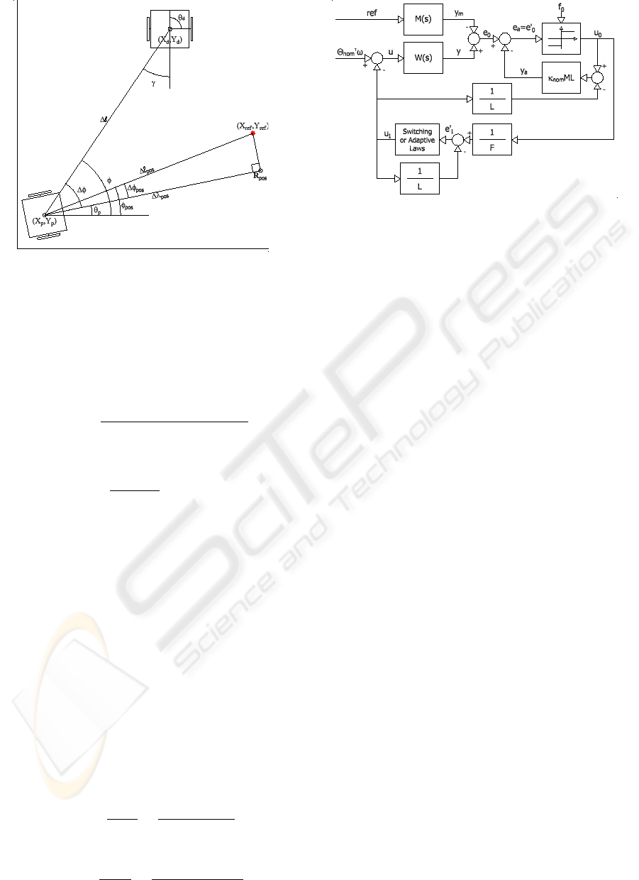
Figure 4: Mobile robot coordinates.
do θ
p
= θ
d
and ∆l → 0, when t → ∞. For this, we
have to do θ
p
→ φ
pos
, φ
pos
→ φ and φ → θ
d
, at the
same time that ∆l → 0 when t → ∞.
Based on the functioning of the positioning con-
troller, it was proposed that each new reference point
has the same distance between robot and desired
point. So
∆l = ∆l
pos
=
q
(x
re f
− x
p
)
2
+ (y
re f
− y
p
)
2
(13)
and that the angle of this point is
tan
−1
y
re f
− y
p
x
re f
− x
p
= φ + γ (14)
To the equations (13) and (13), we obtain the fol-
lowing equations to positioning controller
x
re f
= x
p
+ ∆l · cos(φ +γ)
y
re f
= y
p
+ ∆l · sin(φ +γ)
4.3 Dual-Mode Adaptive Robust
Controller
The DMARC uses the compact VS-MRAC structure,
that was proposed by Araujo and Hsu (Araujo and
Hsu, 1990), changing just the last control signal u
1
(Fig 5) to choose between a VS-MRAC and conven-
tional MRAC controllers.
Consider a linear single-input/single-output time
invariant plant with uncertain parameters and transfer
function,
W (s) = k
p
n
p
(s)
d
p
(s)
=
1
s
2
+ α
1
s + α
2
with input u and output y. The reference model is
M(s) = k
m
n
m
(s)
d
m
(s)
=
k
m
s
2
+ α
m1
s + α
m2
Figure 5: Block diagram of DMRAC controller with n
∗
= 2.
with input re f and output y
m
.
The aim is to find u such that the output error
e
0
= y − y
m
tends to zero asymptotically for arbitrary initial con-
ditions and arbitrary piece-wise continuous uniformly
bounded reference signals re f (t).
Following conventional assumptions are made:
1. the plant is observable, controllable, minimum
phase (n
p
(s) is Hurwitz) and with unknown or un-
certain bounded parameters. d
p
(s) and n
p
(s) are
monics polynomials with degree [d
p
(s)] = 2, de-
gree [n
p
(s)] = 0 and relative degree n
∗
= 2;
2. the reference model is stable and minimum phase
(n
m
(s), d
m
(s) are Hurwitz). d
m
(s) and n
m
(s) are
monics polynomials with relative degree known
(n
∗
) ([M(s)] has the same relative degree than
W (s) and signals sgn(k
p
) = sgn(k
m
) > 0 (positive,
for simplicity).
3. only input/output measurements are used to find
control law u(t).
The following input and output filters are used
˙
Q
1
= −λQ
1
+ gu
˙
Q
2
= −λQ
2
+ gy
where Q
1
,Q
2
∈ ℜ and λ is chosen such that N
m
(s) is
a factor of det(sI − L). The regressor vector is de-
fined as ω
T
=
Q
1
y Q
2
re f
T
, and the control u
is given by
u = Θ
T
ω
where Θ
T
=
Θ
Q1
Θ
n
Θ
Q2
Θ
2n
T
is the adaptive
parameter vector.
Considering the above assumptions exists a uni-
que constant vector Θ
∗
, such that the transfer func-
tion of the closed-loop plant W (S), with u = Θ
∗T
ω,
is M(s) (Matching condition). But θ
∗
is obtained of
exact plant parameters. Usually this is not possible
ICINCO 2007 - International Conference on Informatics in Control, Automation and Robotics
42

in practice, then the Θ is adapted until e
0
→ 0 when
t → ∞, and eventually (under some signal richness
condition) Θ → Θ
∗
.
The vector Θ
∗
is obtained as following
Θ
∗
=
(α
1
− α
m1
)/g
(λ(α
1
− α
m1
) + (α
2
− α
m2
) − α
1
gΘ
∗
v1
)/g
(λ(α
2
− α
m2
) − α
2
gΘ
∗
v1
− k
p
λΘ
∗
n
)/(k
p
· g)
k
m
/k
p
The θ
nom
is a nominal value of adaptive parame-
ter vector (ideally, Θ
nom
= Θ
∗
) and it is calculated as
Q
∗
and based on the decoupled plants (W
S
(s),W
θ
(s))
where α
1
= α
2
= 0.
Suppose that exists a polynomial L(s) = (s + δ)
of degree N = 1 where δ > 0 and δ ∈ ℜ such that
M(s)L(s) is SPR (Strictly Positive Real). Consider
the following auxiliary signal (a prediction of the out-
put error e
0
)
y
a
= MLΘ
2n+1
[L
−1
u − Θ
T
L
−1
ω]
where Θ
2n+1
and Θ are estimates for 1/Θ
∗
2n
and Θ
∗
(Matching parameters), respectively. The following
augmented error is defined
e
a
= (y − y
m
) − y
a
= e
0
− y
a
Narendra proposes the following modification to
guarantee the global stability of the adaptive system
y
a
= ML[Θ
2n+1
(L
−1
Θ
T
− Θ
T
L
−1
)ω
+αe
a
(L
−1
ω)
T
(L
−1
ω)], α > 0
To update Θ and Θ
2n+1
are used the following
adaptive integral laws to MRAC controller
˙
Θ = −e
a
(L−1ω)
˙
Θ
2n+1
= e
a
(L−1Θ
T
− Θ
T
L
−1
)ω
To VS-MRAC controller, we have to introduce the
following filtered signals ξ
0
= L
−1
ω, ξ
1
= ω, χ
0
=
L
−1
u, χ
1
= u.
The upper bounds are defined by
Θ
11
> |Θ
∗
Q1
− Θ
nom,Q1
| Θ
12
> |Θ
∗
n
− Θ
nom,n
|
Θ
13
> |Θ
∗
Q2
− Θ
nom,Q2
| Θ
14
> |Θ
∗
2n
− Θ
nom,2n
|
Θ
1
=
Θ
11
Θ
12
Θ
13
Θ
14
T
Θ
0 j
> ρ · Θ
1 j
, j = 1, 2,3,4
κ >
κ
∗
− κ
nom
κ
nom
where ρ = κ
∗
/κ
nom
(ideally ρ = 1) and κ
nom
is a nom-
inal value for k
∗
= 1/Θ
∗
2n
(it is assumed k
nom
6= 0).
Further, it is defined
u
nom
= Θ
T
nom
ω (15)
We have plants with n
∗
= 2 and in this case, a VS-
MRAC structure, needs a chain of auxiliary errors to
get the matching condition. The switching laws are
chosen so that the auxiliary errors e
0
i
(i = 0,1) become
sliding modes after some finite time. The equivalent
controls ((u
i
)
eq
) are, in practice, obtained of (u
i
) by
means of a low pass filter (F) with high enough cut-
off frequency.
To adjust the DMARC controller an expression
for the µ parameter, based on the idea of the Takagi-
Sugeno model, was used. This expression is given by
(16), where ` is a parameter to be adjusted.
µ = e
−(e
0
1
)
2
/`
(16)
Notice that when e
0
1
→ 0, µ → 1 and the algo-
rithm is the MRAC. When e
0
1
becomes reasonably
high, µ assumes a value sufficiently small, tending to
the VSMRAC algorithm. The ` parameter has a great
importance in the transition between MRAC and VS-
MRAC. If ` is small the VS-MRAC action will be big.
The DMARC algorithm applied to plants with rel-
ative degree n
∗
= 2 is summarized in the Table 1.
Table 1: Algorithm of DMARC controller.
u = −u
1
+ u
nom
y
a
= κ
nom
ML · [u
0
− L
−1
u
1
]
e
0
0
= e
a
= e
0
− y
a
(u
0
)
eq
= F
−1
(u
0
)
e
0
1
= (u
0
)
eq
− L
−1
(u
1
)
f
0
= κ|χ
0
− Θ
T
nom
ξ
0
| + Θ
T
0
· |ξ
0
|
f
1
= Θ
T
1
· |ξ
1
|
u
0
= f
0
· sgn(e
0
0
)
u
1
= −Θ
T
1
ω
µ
˙
Θ
1
= −αΘ
1
− αΘ
1
· sgn(e
0
1
ω), α > 0
5 RESULTS
The result showed in this paper is based on simulation
of a micro robot soccer structure. The simulated result
considers the main nonlinearities (see (Laura et al.,
2006)) as dead zone between ±150mV and saturation
to values out of ±10V . It also has noise in input and
output signals. The noise was calculated by a ran-
dom variable with a normal distribution of probabil-
ity. To inputs noises (e
d
,e
e
) we have values between
±100mV . To output noises (x
p
, y
p
and θ
p
) we have
values between ±1cm to cartesian points and ±8, 5
o
to angle.
The unknown parameters are in the dynamic mo-
del, and they are obtained of the exact mobile robot
A DUAL MODE ADAPTIVE ROBUST CONTROLLER FOR DIFFERENTIAL DRIVE TWO ACTUATED WHEELED
MOBILE ROBOT
43
model with a normal distribution random variable of
probability between 1% and 10%. The parameters
used in the simulation are of a realistic robot, that is
not symmetrical.
A controller DMRAC is applied to each plant
(W
S
(s) and W
θ
(s) with relative degree → n
∗
= 2).
Choosing a reference model to each plant, we have
M
S
(s) =
2.25
s
2
+ 3s + 2.25
M
θ
(s) =
100
s
2
+ 20s + 100
and as filters
˙
Q
S1
= −1.5Q
S1
+ 1.5U
S
˙
Q
S2
= −1.5Q
S2
+ 1.5S
˙
Q
θ1
= −10Q
θ1
+ 10U
θ
˙
Q
θ2
= −10Q
θ2
+ 10θ
p
We choose the polynomial L
S
(s) = s + 1.5 to
DMARC
S
with F = 22s + 1, `
S
= 0.7551, α
S
= 0.05
and
Θ
S,nom
= [ −2.0 −6.75 4.5 2.25 ]
T
Θ
S,1
= [ 2.420 13.282 2.657 0.024 ]
T
We choose the polynomial L
θ
(s) = s + 10 to
DMARC
θ
with F = 56s + 1, `
θ
= 0.0051, α
θ
= 0.05
and
Θ
θ,nom
= [ −2.0 −300.0 200.0 9.7 ]
T
Θ
θ,1
= [ 0.073 101.161 175.750 0.1 ]
T
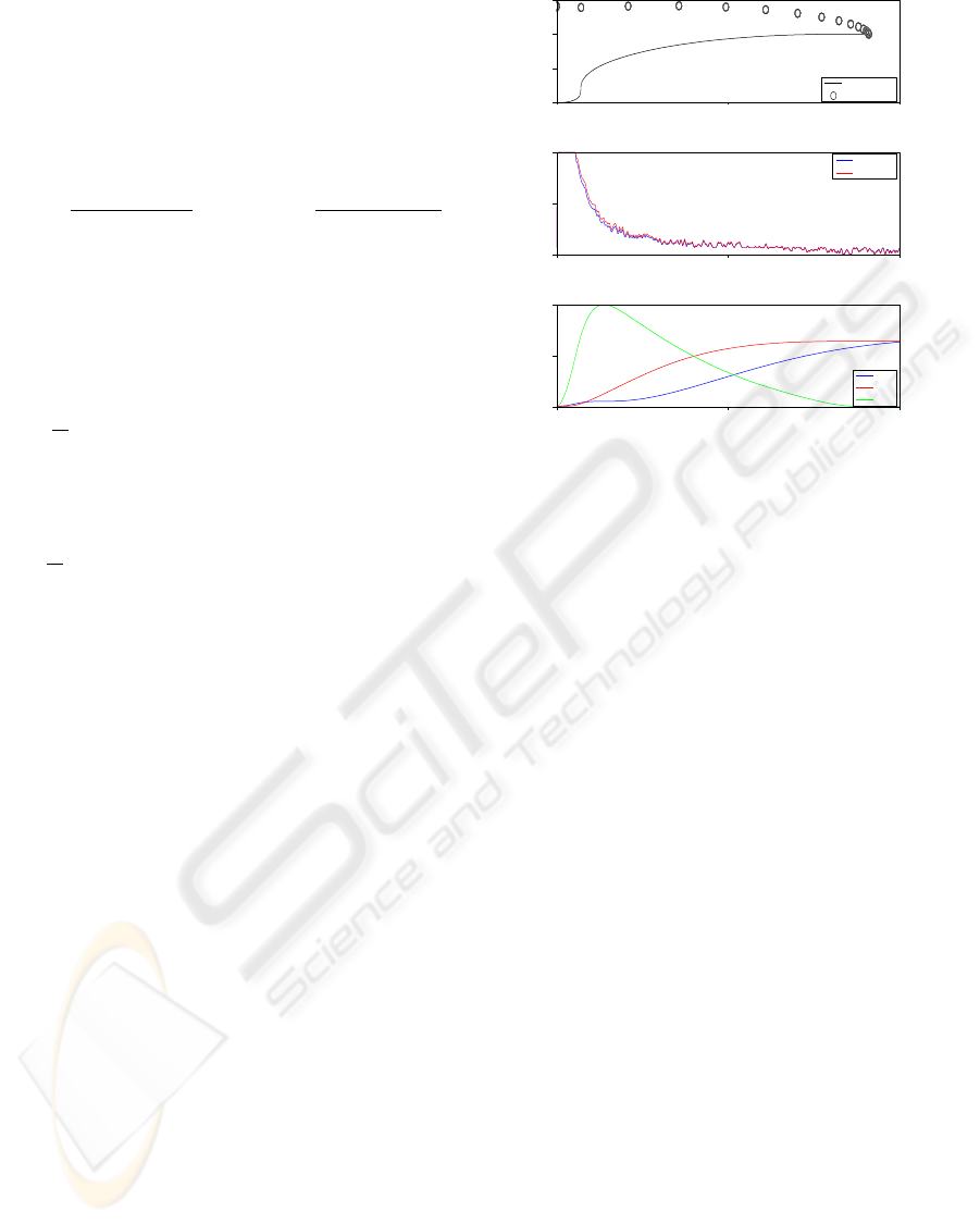
The Fig. 6 shows a simulation result of the closed
loop system. The robot going from the initial point
0 0 0
T
to desired point
1 1 0
T
. When the
robot reaches a circle of 1cm radius with center in de-
sired point, it’s considered that the task was accom-
plished. The controller shows a good transient behav-
ior that means in 3.49s the robot reaches the desired
position without vibrations.
The simulation result is closed to real physical
systems, so it includes the main nonlinearities, a plant
with unknown parameters, bounded disturbances in
the absolute positioning system and in motors driver
system. It uses a sampling interval of 10ms. These
facts did not affect the closed loop system behavior.
In the Fig. 6 is possible identify the functioning
of the DMARC controller. When the error is big a
DMARC operates as VS-MRAC and when the error
is small the DMRAC operates as MRAC.
6 CONCLUSIONS
In this paper a controller that decouples multivariable
system into two monovariable systems was proposed.
For each monovariable system an adaptive robust con-
troller is applied to get desired responses.
The closed loop system with the proposed con-
troller presented a good transient response and robust-
ness to disturbances and errors in the absolute posi-
tioning system and in driver system.
−0.00 0.55 1.10
0.0
0.5
1.0
1.5
Robot Trajectory
x
y
Trajectory
Reference Point
0.00 1.75 3.49
−0.82
4.59
10.00
Motors Signals
t
x
Right Motor
Left Motor
0.00 1.75 3.49
−0.02
0.77
1.56
X,Y,Angle Evolution
t
X
Y
Angle
Figure 6: Robot signals (control signal and output plant).
REFERENCES
Araujo, A. D. and Hsu, L. (1990). Further developments in
variable structure adaptive control based only on in-
put/output measurements. volume 4, pages 293–298.
11th IFAC World Congress.
Chang, C., Huang, C., and Fu, L. (2004). Adaptive track-
ing control of a wheeled mobile robot via uncalibrated
camera system. volume 6, pages 5404–5410. IEEE
International Conference on Systems, Man and Cy-
bernetics.
Cunha, C. D. and Araujo, A. D. (2004). A dual-mode adap-
tive robust controller for plants with arbitrary relative
degree. Proceedings of the 8th International Work-
shop on Variable Structure Systems, Spain.
Dixon, W. E., Dawson, D. M., Zergeroglu, E., and Behal,
A. (2001). Adaptive tracking control of a wheeled
mobile robot via uncalibrated camera system. IEEE
Transactiond on on Systems, Man and Cybernetics,
31(3):341–352.
Hirschorn, R. M. (1979). Invertibility of multivariable non-
linear control systems. IEEE Transactions on Auto-
matic Control, AC-24:855–865.
Hsu, L. and Costa, R. R. (1989). Variable structure model
reference adaptive control using only input and out-
put measurements - part 1. International Journal of
Control, 49(02):399–416.
Laura, T. L., Cerqueira, J. J. F., Paim, C. C., Pomlio, J. A.,
and Madrid, M. K. (2006). Modelo dinmico da es-
trutura de base de robs mveis com incluso de no lin-
earidades - o desenvolvimento do modelo. volume 1,
pages 2879–2884. Anais do XVI Congresso Brasileiro
de Automtica, 2006.
ICINCO 2007 - International Conference on Informatics in Control, Automation and Robotics
44
