GEOMETRIC CONTROL OF A BINOCULAR HEAD
Eduardo Bayro-Corrochano and Julio Zamora-Esquivel
Department of Electrical Engineering and Computer Science
CINVESTAV, unidad Guadalajara. Jalisco, Mexico
Keywords:
Conformal Geometry, Kinematics, Tracking.
Abstract:
In this paper the authors use geometric algebra to formulate the differential kinematics of a binocular robotic
head and reformulate the interaction matrix in terms of the lines that represent the principal axes of the camera.
This matrix relates the velocities of 3D objects and the velocities of their images in the stereo images. Our
main objective is the formulation of a kinematic control law in order to close the loop between perception and
action, which allows to perform a smooth visual tracking.
1 INTRODUCTION
In this work we formulate the problem of visual track-
ing and design a control law by velocity feedback
that allows us to close the loop between perception
and action. Geometric algebra allow us to work
with geometric entities like points, lines and planes
and helps in the representation of rigid transforma-
tions. In this mathematical framework we straightfor-
wardly formulate the direct and differential kinemat-
ics of robotic devices like the binocular robot head.
On the other hand we show a reformulation of vi-
sual Jacobean which relates the velocity of a tridimen-
sional object with the velocity of its projection onto
the stereo camera images. Finally we write an ex-
pression that relates the joint velocities in the pan-tilt
unit and velocities of the points in the camera image.
We start this work presenting a brief description of
the geometric entities and conformal transformations
them we show the kinematics of a pan-tilt unit and
formulate its control law.
In contrast to other authors like (C. Canudas de
Wit and Bastin, 1996), (Ruf, 2000) or (Kim Jung-Ha.,
1990) we will use multivectors instead of matrices to
formulate the control law it reduces the computation
and improve the performance of the controller.
2 GEOMETRIC ALGEBRA: AN
OUTLINE
Let
G
n
denote the geometric algebra of n-dimensions,
this is a graded linear space. As well as vector
addition and scalar multiplication we have a non-
commutative product which is associative and dis-
tributive over addition – this is the geometric or Clif-
ford product.
The inner product of two vectors is the standard
scalar or dot product and produces a scalar. The outer
or wedge product of two vectors is a new quantity
which we call a bivector. We think of a bivector as a
oriented area in the plane containing a and b, formed
by sweeping a along b.
Thus, b∧a will have the opposite orientation mak-
ing the wedge product anti-commutative. The outer
product is immediately generalizable to higher di-
mensions – for example, (a ∧ b) ∧ c, a trivector, is
interpreted as the oriented volume formed by sweep-
ing the area a∧ b along vector c. The outer product of
k vectors is a k-vector or k-blade, and such a quantity
is said to have grade k. A multivector (linear combi-
nation of objects of different type) is homogeneous if
it contains terms of only a single grade.
2.1 The Geometric Algebra of n-D
Space
In this paper we will specify a geometric algebra
G
n
of the n dimensional space by G
p,q,r
, where p, q and r
183
Bayro-Corrochano E. and Zamora-Esquivel J. (2007).
GEOMETRIC CONTROL OF A BINOCULAR HEAD.
In Proceedings of the Fourth International Conference on Informatics in Control, Automation and Robotics, pages 183-188
DOI: 10.5220/0001628001830188
Copyright
c
 SciTePress

stand for the number of basis vector which squares to
1, -1 and 0 respectively and fulfill n = p+q+ r.
We will use e
i
to denote the vector basis i. In a Ge-
ometric algebra G
p,q,r
, the geometric product of two
basis vector is defined as
e
i
e
j
=





1 for i = j ∈ 1, ··· , p
−1 for i = j ∈ p+ 1, ·· · , p+ q
0 for i = j ∈ p+ q+ 1, ·· · , p+ q+ r.
e
i
∧ e
j
for i 6= j
This leads to a basis for the entire algebra:
{1}, {e
i
}, {e
i
∧ e
j
}, {e
i
∧ e
j
∧ e
k
}, . . . , {e
1
∧ e
2
∧ . . . ∧ e
n
} (1)
Any multivector can be expressed in terms of this
basis.
3 CONFORMAL GEOMETRY
Geometric algebra G
4,1
can be used to treat confor-
mal geometry in a very elegant way. To see how this
is possible, we follow the same formulation presented
in (H. Li, 2001) and show how the Euclidean vector
space R
3
is represented in R
4,1
. This space has an or-
thonormal vector basis given by {e
i
} and e
ij
= e
i
∧ e
j
are bivectorial basis and e
23
, e
31
and e
12
correspond to
the Hamilton basis. The unit Euclidean pseudo-scalar
I
e
:= e
1
∧ e
2
∧ e
3
, a pseudo-scalar I
c
:= I
e
E and the
bivector E := e
4
∧ e
5
= e
4
e
5
are used for computing
the inverse and duals of multivectors.
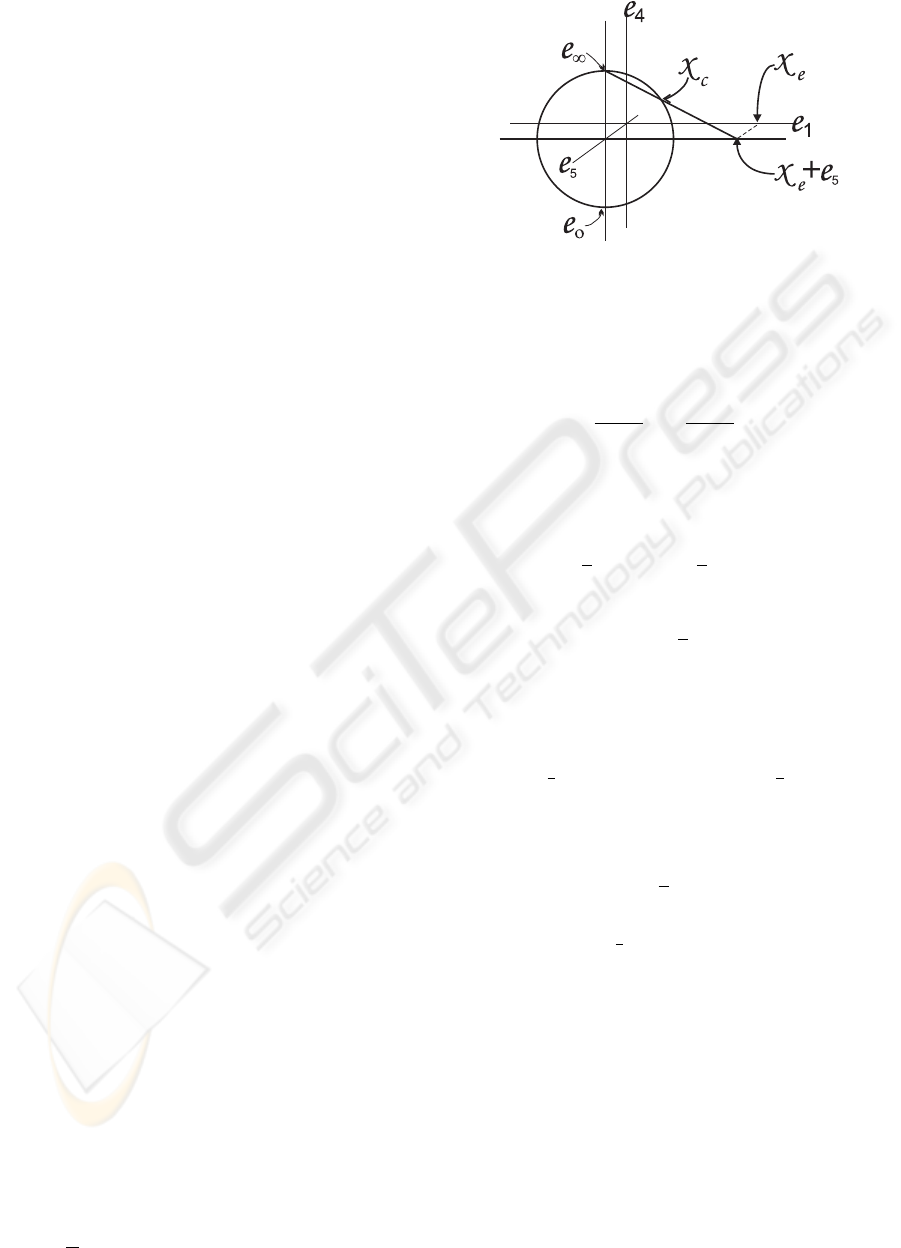
3.1 The Stereographic Projection
The conformal geometry is related to a stereographic
projection in Euclidean space. A stereographic pro-
jection is a mapping taking points lying on a hyper-
sphere to points lying on a hyperplane. In this case,
the projection plane passes through the equator and
the sphere is centered at the origin. To make a projec-
tion, a line is drawn from the north pole to each point
on the sphere and the intersection of this line with the
projection plane constitutes the stereographic projec-
tion.
For simplicity, we will illustrate the equivalence
between stereographic projections and conformal ge-
ometric algebra in R
1
. We will be working in R
2,1
with the basis vectors {e
1
, e
4
, e
5
} having the usual
properties. The projection plane will be the x-axis
and the sphere will be a circle centered at the origin
with unitary radius.
Given a scalar x
e
representing a point on the x-
axis, we wish to find the point x
c
lying on the circle
that projects to it (see Figure 1). The equation of the
line passing through the north pole and x
e
is given by
f(x) = −
1
x
e
x + 1 and the equation of the circle x
2
+
Figure 1: Stereographic projection for 1-D.
f(x)
2
= 1. Substituting the equation of the line on the
circle, we get the point of intersection x
c
which can be
represented in homogeneous coordinates as the vector
x
c
= 2
x
e
x
2
e
+ 1
e
1
+
x
2
e
− 1
x
2
e
+ 1
e
4
+ e
5
. (2)
From (2) we can infer the coordinates on the circle for
the point at infinity as
e
∞
= lim
x
e
→∞
{
x
c
}
= e
4
+ e
5
, (3)
e
o
=
1
2
lim
x
e
→0
{
x
c
}
=
1
2
(−e
4
+ e
5
), (4)
Note that (2) can be rewritten to
x
c
= x
e
+
1
2
x
2
e
e
∞
+ e
o
, (5)
3.2 Spheres and Planes
The equation of a sphere of radius ρ centered at point
p
e
∈ R
n
can be written as (x
e
− p
e
)
2
= ρ
2
. Since
x
c
· y
c
= −
1
2
(x
e
− y
e
)
2
and x
c
· p
c
= −
1
2
ρ
2
., we can
rewrite the formula above in terms of homogeneous
coordinates as. Since x
c
· e
∞
= −1 we can factor the
expression above to
x
c
· (p
c
−
1
2
ρ
2
e
∞
) = 0. (6)
Which finally yields the simplified equation for the
sphere as s = p
c
−
1
2
ρ
2
e
∞
. Note from this equation
that a point is just a sphere with zero radius. Alterna-
tively, the dual of the sphere is represented as 4-vector
s
∗
= sI
c
. The advantage of the dual form is that the
sphere can be directly computed from four points as
s
∗
= x
c
1
∧ x
c
2
∧ x
c
3
∧ x
c
4
. (7)
If we replace one of these points for the point at infin-
ity we get the equation of a plane
π
∗
= x
c
1
∧ x
c
2
∧ x
c
3
∧ e
∞
. (8)
So that π becomes in the standard form
π = I
c
π
∗
= n+ de
∞
(9)
Where n is the normal vector and d represents the
Hesse distance.
ICINCO 2007 - International Conference on Informatics in Control, Automation and Robotics
184

3.3 Circles and Lines
A circle z can be regarded as the intersection of two
spheres s
1
and s
2
as z = (s
1
∧ s
2
). The dual form of
the circle can be expressed by three points lying on it
z
∗
= x
c
1
∧ x
c
2
∧ x
c
3
. (10)
Similar to the case of planes, lines can be defined
by circles passing through the point at infinity as:
L
∗
= x
c
1
∧ x
c
2
∧ e
∞
. (11)
The standard form of the line can be expressed by
L = l + e
∞
(t · l), (12)
the line in the standard form is a bivector, and it has
six parameters (Plucker coordinates).
4 RIGID TRANSFORMATIONS
We can express rigid transformations in conformal ge-
ometry carrying out reflections between planes.
4.0.1 Reflection
The reflection of conformal geometric entities help us
to do any other transformation. The reflection of a
point x respect to the plane π is equal x minus twice
the direct distance between the point and plane see
the image 2, that is x = x− 2(π·x)π
−1
to simplify this
expression recalling the property of Clifford product
of vectors 2(b· a) = ab+ ba.
Figure 2: Reflection of a point x respect to the plane π.
For any geometric entity Q, the reflection respect to
the plane π is given by
Q
′
= πQπ
−1
(13)
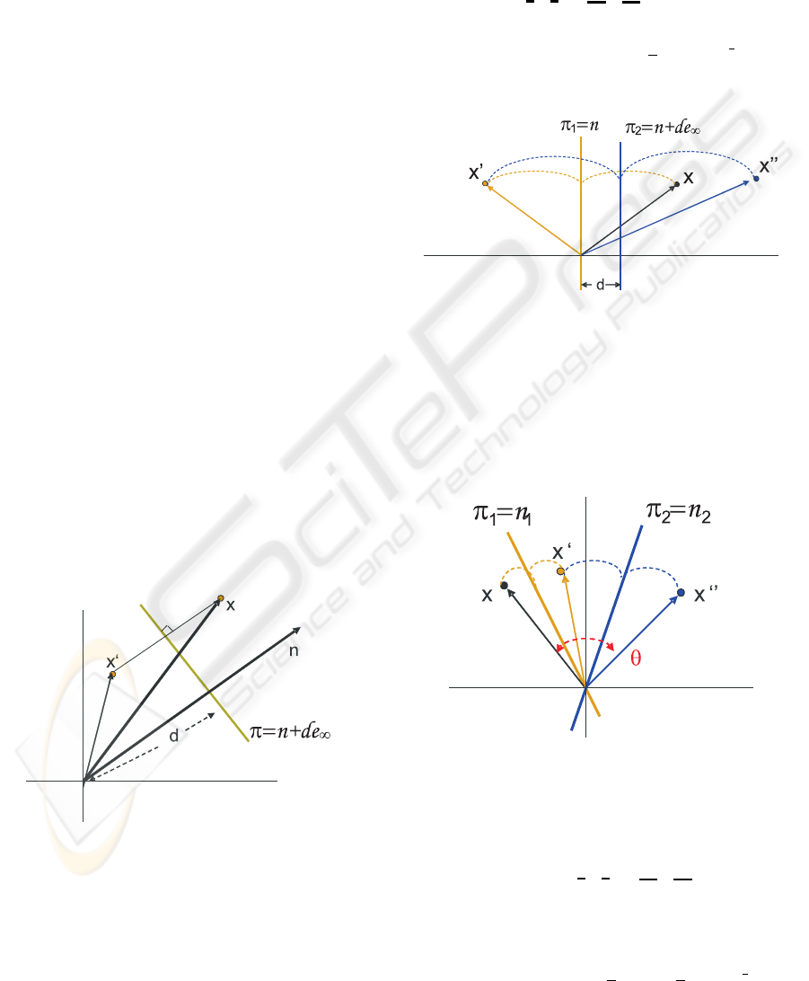
4.0.2 Translation
The translation of conformal entities can be done by
carrying out two reflections in parallel planes π
1
and
π
2
see the image (3), that is
Q
′
= (π
2
π
1
)
|
{z}
T
a
Q(π
−1
1
π
−1
2
)
|
{z }
e
T
a
(14)
T
a
= (n+ de
∞
)n = 1+
1
2
ae
∞
= e
−
a
2
e
∞
(15)
With a = 2dn.
Figure 3: Reflection about parallel planes.
4.0.3 Rotation
The rotation is the product of two reflections between
nonparallel planes, (see image (4))
Figure 4: Reflection about nonparallel planes.
Q
′
= (π
2
π
1
)
|
{z}
R
θ
Q(π
−1
1
π
−1
2
)
|
{z }
f
R
θ
(16)
Or computing the conformal product of the normals
of the planes.
R
θ
= n
2
n
1
= Cos(
θ
2
) − Sin(
θ
2
)l = e
−
θ
2
l
(17)
GEOMETRIC CONTROL OF A BINOCULAR HEAD
185

With l = n
2
∧ n
1
, and θ twice the angle between the
planes π
2
and π
1
. The screw motion called motor re-
lated to an arbitrary axis L is M = TR
e
T
Q
′
= (TR
e
T)
|
{z }
M
θ
Q((T
e
R
e
T))
|
{z }
f
M
θ
(18)
M
θ
= TR
e
T = Cos(
θ
2
) − Sin(
θ
2
)L = e
−
θ
2
L
(19)
4.1 Kinematic Chains
The direct kinematics for serial robot arms is a succes-
sion of motors as you can see in (Bayro-Corrochano
and Kahler, 2000) and it is valid for points, lines,
planes, circles and spheres.
Q
′
=
n
∏
i=1
M
i
Q
n
∏
i=1
e
M
n−i+1
(20)
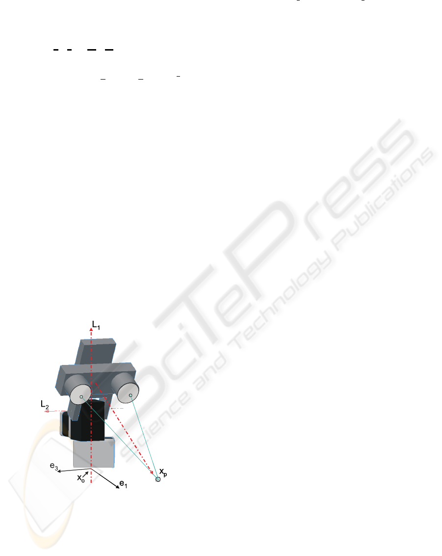
5 DIRECT KINEMATICS OF A
PAN-TILT UNIT
We implement algorithm for the velocity control of a
pan-tilt unit (PTU Fig. 5) assuming three degree of
freedom. We consider the stereo depth as one virtual
D.O.F. thus the PTU has a similar kinematic behavior
as a robot with three D.O.F.
Figure 5: Pan tilt unit.
In order to carry out a velocity control, we need
first to compute the direct kinematics, this is very easy
to do, as we know the axis lines:
L
1
= −e
31
(21)
L
2
= e
12
+ d
1
e
1
e
∞
(22)
L
3
= e
1
e
∞
(23)
Since M
i
= e
−
1
2
q
i
L
i
and
e
M
i
= e
1
2
q
i
L
i
, The position
of end effectors is computed as
x
p
(q) = x
′
p
= M
1
M
2
M
3
x
p
e
M
3
e
M
2
e
M
1
, (24)
The state variable representation of the system is
as follows







˙x
′
p
= x
′
·

L
′
1
L
′
2
L
′
3



u
1
u
2
u
3


y = x
′
p
(25)
where the position of end effector at home po-
sition x
p
is the conformal mapping of x
p
e
= d
3
e
1
+
(d
1
+ d
2
)e
2
(see eq. 5), the line L
′
i
is the current posi-
tion of L
i
and u
i
is the velocity of the i-junction of the
system. As L
3
is an axis at infinity M
3
is a translator,
that is, the virtual component is a prismatic junction.
5.1 Exact Linearization via Feedback
Now the following state feedback control law is cho-
sen in order to get a new linear an controllable system.


u
1
u
2
u
3


=

x
′
p
· L
′
1
x
′
p
· L
′
2
x
′
p
· L
′
3

−1


v
1
v
2
v
3


(26)
WhereV = (v
1
, v
2
, v
3
)
T
is the new input to the lin-
ear system, then we rewrite the equations of the sys-
tem

˙x
′
p
= V
y = x
′
p
(27)
5.2 Asymptotical Output Tracking
The problem of follow a constant reference x
t
is
solved computing the error between end effectors po-
sition x
′
p
and the target position x
t
as e
r
= (x
′
p
∧x
t
)·e
∞
,
the control law is then given by.
V = −ke (28)
This error is small if the control system is doing
it’s job, it is mapped to an error in the joint space using
the inverse Jacobian.
U = J
−1
V (29)
Doing the Jacobian J = x
′
p
·

L
′
1
L
′
2
L
′
3

j
1
= x
′
p
· (L
1
) (30)
j
2
= x
′
p
· (M
1
L
2
e
M
1
) (31)
j
3
= x
′
p
· (M
1
M
2
L
3
e
M
2
e
M
1
) (32)
ICINCO 2007 - International Conference on Informatics in Control, Automation and Robotics
186

Once that we have the Jacobian is easy to compute
the dq
i
using the crammer’s rule.


u
1
u
2
u
3


= ( j
1
∧ j
2
∧ j
3
)
−1
·


V ∧ j
2
∧ j
3
j
1
∧V ∧ j
3
j
1
∧ j
2
∧V


(33)
This is possible because j
1
∧ j
2
∧ j
3
= det(J)I
e
.
Finally we have dq
i
which will tend to reduce these
errors.
5.3 Visual Jacobian
A point in the image is given by s = (x, y)
T
whereas
a 3-D point is represented as X. The relationship be-
tween ˙s and
˙
S is called visual Jacobian.
Taking a camera in general position his projection
matrix is represented by the planes π
1
, π
2
y π
3
more
details in (Hartley and Zisserman, 2000).
P =


π
1
π
2
π
3


, (34)
The point X is projected in the image in the point
s =
π
1
·X
π
3
·X
π
2
·X
π
3
·X
!
(35)
To simplify the explanation the x variable is intro-
duced and his time derivative ˙x defined as
x =


π
1
· X
π
2
· X
π
3
· X


˙x =


π
1
·
˙
X
π
2
·
˙
X
π
3
·
˙
X


(36)
Now s is given by s
1
=
x
1
x
3
and his derivative
˙s
1
= ˙x
1
1
x
3
+ x
1

− ˙x
3
x
2
3

(37)
˙s
1
=
x
3
˙x
1
− x
1
˙x
3
x
2
3
(38)
By sustitution of x and ˙x in the equation 38 is obtained
˙s
1
= κ[(π
3
· X)π
1
− (π
1
· X)π
3
] ·
˙
X (39)
˙s
1
= κ[X ·(π
3
∧ π
1
)] ·
˙
X (40)
where κ =
1
x
2
3
. Doing the same steps for s
2
it possible
to write the equation
˙s = κX ·

π
1
∧ π
3
π
2
∧ π
3

·
˙
X (41)
Geometrically π
1
∧π
3
represents a line of intersection
of the planes π
1
and π
3
. Denoting by L
x
and L
y
the
lines of this intersection as
L
x
= π
1
∧ π
3
(42)
L
y
= π
2
∧ π
3
(43)
It is posible to rewrite 41 as
˙s = κX ·

L
x
L
y

·
˙
X (44)
In order to close the loop between the perception
and action, the relationship between velocities in the
points of the image and the velocities in the joints of
the pan-tilt unit is computed.
Taking the equation of differential kinematics 25
and visual Jacobian 44 it is possible to write a new
expression
˙s = κ

(X
′
· L
′
x
) · (X
′
· L
′
1
) (X
′
· L
′
x
) · (X
′
· L
′
2
)

X
′
· L
′
y

· (X
′
· L
′
1
)

X
′
· L
′
y

· (X
′
· L
′
2
)

˙q (45)
We can write a similar expression using the differen-
tial kinematics of the Barrett Hand. The equation 45
is very useful to design a control law to track an object
or to grasp it.
5.4 Exact Linearization via Feedback
Now the following state feedback control law is cho-
sen in order to get a new linear an controllable sys-
tem.

u
1
u
2

=

(X
′
· L
′
x
) ·

X
′
· L
′
1

(X
′
· L
′
x
) ·

X
′
· L
′
2


X
′
· L
′
y

·

X
′
· L
′
1
 
X
′
· L
′
y

·

X
′
· L
′
2


−1

v
1
v
2

Where V = (v
1
, v
2
)
T
is the new input to the linear
system, then we rewrite the equations of the system

˙s
′
p
= V
y = s
′
p
(46)
5.5 Experimental Results
In this experiment the binocular head should
smoothly track a target. The figure (6) show the 3D
coordinates of the focus of attention. The figure (7)
show examples of the image sequence. We can see
that the curves of the 3D object trajectory are very
rough, however the control rule manages to keep the
trajectory of the pan-tilt unit smooth.
In the experiment the coordinate system is in the
center of the camera. Then the principal planes of the
camera are given by
π
1
= f
x
e
1
+ x
o
e
3
(47)
π
2
= f
y
e
2
+ y
o
e
3
(48)
π
3
= e
3
(49)
whre f
x
, f
y
, x
o
y y
o
are the camera’s parameters. Us-
ing this planes we compute the lines L
x
y L
y
, by the
way the axis of the pan-tilt are known.
L
1
= e
23
+ d
1
e
2
(50)
L
2
= e
12
+ d
2
e
2
(51)
GEOMETRIC CONTROL OF A BINOCULAR HEAD
187

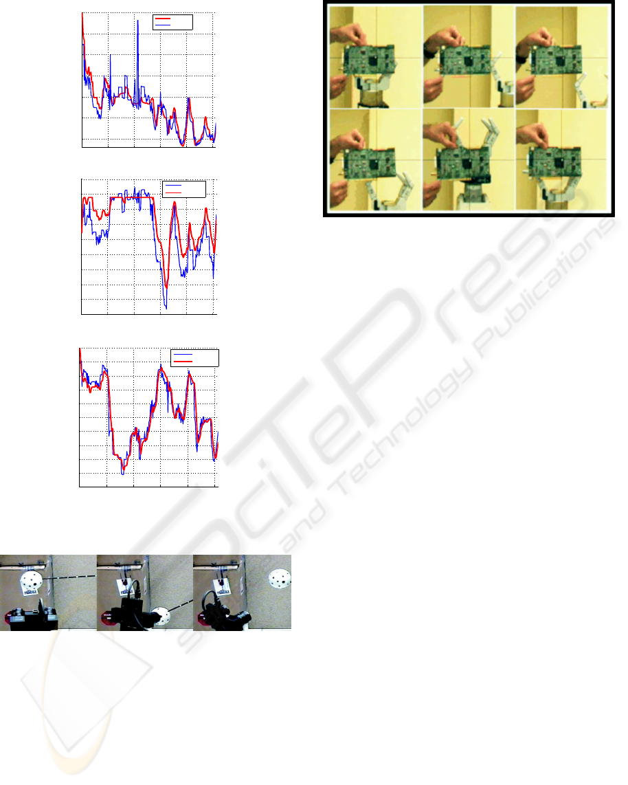
0 50 100 150 200 250
−30
−25
−20
−15
−10
−5
0
x−PTU
x−Object
0 50 100 150 200 250
−15
−10
−5
0
5
10
15
20
25
30
y−Object
y−PTU
0 50 100 150 200 250
−20
−15
−10
−5
0
5
10
15
20
25
30
z−Object
z−PTU
Figure 6: x, y and z coordinate of the focus of attention.
Figure 7: Sequence of tracking.
Note that the tilt axis is called L
1
and the pan axis
is L
2
, because the coordinate system is in the camera.
also L
′
2
is a function of the tilt angle L
′
2
= M
1
L
2
˜
M
1
with M
1
= cos(θ
tilt
)+sen(θ
tilt
)L
1
. In this experiment
a point over the boar was selected and using the KLT
algorithm was tracked the displacement in the image
is transformed to velocities of the pan-tilt’s joint using
the visual-mechanical Jacobean Eq. 45.
As result in the image (8) we can see a sequence
of pictures captured by the robot. In these images the
position of the board do not change while the back-
ground is in continuous change.
Figure 8: Sequence of tracking.
6 CONCLUSION
The authors show that is possible and easy to write
a control law using the lines of the camera’s axes as
bivectors (Plcker coordinates) in the conformal geom-
etry instead of the interaction matrix. This formula-
tion combines the information of the camera’s param-
eters with the axes of the pan tilt unit in order to create
a matrix of the visual-mechanical Jacobian useful to
write a velocity control law. The experiments confirm
the effectiveness of our approach.
REFERENCES
Bayro-Corrochano, E. and Kahler, D. (2000). Motor algebra
approach for computing the kinematics of robot ma-
nipulators. In Journal of Robotic Systems. 17(9):495-
516.
C. Canudas de Wit, B. S. and Bastin, G. (1996). Theory of
Robot Control. Springer, Berlin, 1st edition.
H. Li, D. Hestenes, A. R. (2001). Generalized Homoge-
neous coordinates for computational geometry. pages
27-52, in (Somer, 2001).
Hartley and Zisserman, A. (2000). Multiple View Geometry
in Computer Vision. Cambridge University Press, UK,
1st edition.
Kim Jung-Ha., K. V. R. (1990). Kinematics of robot manip-
ulators via line transformations. In Journal of Robotic
Systems. pp. 647-674.
Ruf, A. (2000). Closing the loop between articulated mo-
tion and stereo vision: a projective approach. In PhD.
Thesis, INP, GRENOBLE.
Somer, G. (2001). Geometric Computing with Clifford Al-
gebras. Springer-Verlag, Heidelberg, 2nd edition.
ICINCO 2007 - International Conference on Informatics in Control, Automation and Robotics
188