
SCHEDULING OF MULTI-PRODUCT BATCH PLANTS USING
REACHABILITY ANALYSIS OF TIMED AUTOMATA MODELS
Subanatarajan Subbiah, Sebastian Panek, Sebastian Engell
Process Control Laboratory (BCI-AST), University of Dortmund, 44221 Dortmund, Germany
Olaf Stursberg
Industrial Automation Systems (EI-LSR), Technical University of Muenchen, Muenchen, Germany
Keywords:
Scheduling, timed automata, reachability analysis, multi-product batch plant.
Abstract:
Standard scheduling approaches in process industries are often based on algebraic problem formulations
solved as MI(N)LP optimization problems to derive production schedules. To handle such problems tech-
niques based on timed automata have emerged recently. This contribution reports on a successful application
of a new modeling scheme to formulate scheduling problems in process industries as timed automata (TA)
models and describes the solution technique to obtain schedules using symbolic reachability analysis. First,
the jobs, resources and additional constraints are modeled as sets of synchronized timed automata. Then, the
individual automata are composed by parallel composition to form a global automaton which has an initial
location where no jobs have been started and at least one target location where all jobs have been finished. A
cost optimal symbolic reachability analysis is performed on the composed automaton to derive schedules. The
main advantage of this approach over other MILP techniques is the intuitive graphical and modular modeling
and the ability to compute better solutions within reasonable computation time. This is illustrated by a case
study.
1 INTRODUCTION
Scheduling has applications in many fields and one
among them are the chemical industries employed
with multi-product batch plants. Multi-product batch
plants in contrast to continuous plants offer the ad-
vantage of an increased flexibility with respect to the
variation of the products, the volume of production,
and the range of recipes that can be processed by
the equipment. This flexibility makes the scheduling
task challenging. The scheduler has to take a large
number of decisions to answer questions of what,
when, where and how to produce the products in or-
der to satisfy the market demand. The scheduling
task is particularly challenging due to numerous con-
straints arising from process topology, the interlinks
between pieces of equipment, inventory policies, ma-
terial transfers, batch sizes, batch processing times,
demand patterns, changeover procedures, resource
and time constraints, cost functions and degrees of
uncertainty. Many scientists in the process logistics
community have contributed approaches to model and
solve such problems (Kallrath, 2002). In most promi-
nent approaches the problem is specified using the
frameworks of State Task Networks (STN) or Re-
source Task Networks (RTN) (Pantelides, 1994), fur-
ther transformed to an optimization problem modeled
as a mixed integer program (MILP or MINLP) and
solved using state-of-the art solvers such as CPLEX,
XPRESS-MP, etc. The modeling of mathematical
optimization problems is generally cumbersome, te-
dious and requires not only experience in algebraic
modeling but also a deep knowledge of the solver and
its internal algorithms.
Recently, techniques based on reachability analy-
sis for timed automata to solve scheduling problems
have gained attention. The framework of TA has been
originally proposed by (Alur and Dill, 1994) to model
timed systems with discrete dynamics. Many power-
ful tools for the modeling and analysis of real-time
systems such as UPPAAL, IF, KRONOS and TAOPT
have emerged. The authors of (Abdeddaim and Maler,
2001) have proposed to use TA to solve job-shop
scheduling problems based on the symbolic reacha-
141
Subbiah S., Panek S., Engell S. and Stursberg O. (2007).
SCHEDULING OF MULTI-PRODUCT BATCH PLANTS USING REACHABILITY ANALYSIS OF TIMED AUTOMATA MODELS.
In Proceedings of the Fourth International Conference on Informatics in Control, Automation and Robotics, pages 141-148
DOI: 10.5220/0001627501410148
Copyright
c
SciTePress

bility analysis of TA. Promising results on challeng-
ing benchmark instances in job-shops were reported
in (Panek et al., 2006). The particular appeal of this
approach comes from the modular and partly graph-
ical modeling which enables inexperienced users to
build models. Another advantage is the availability
of powerful search algorithms that can easily be mod-
ified and extended for special purposes. Similar to
other approaches the reachability analysis of TA also
suffers from the drastic increase in the computational
cost with an increase in the problem size. The prob-
lem of state-space explosion in TA models can be re-
duced to some extent by state-space reduction tech-
niques (Panek et al., 2007), but arises again when the
problem instance is scaled. An advantage of the TA-
based approach is that good, though not provable op-
timal solutions are often found relatively quickly.
The structure of the rest of this paper is as fol-
lows: In Section 2, Resource Task Networks (RTN)
are introduced as the basic model for specifying batch
scheduling problems. Section 3 explains how the
RTN model can be translated into TA, and how the
corresponding scheduling problem can be solved by
symbolic reachability analysis. In section 4, differ-
ent greedy strategies to reduce the solution space are
explained. The description of the case study and the
results of the experiments for the example considered
are provided in section 5. The paper closes with con-
clusions and an outlook.
2 MODELING WITH RTN
In the context of mathematical programming, STN
and RTN serve as starting points for formulating in-
tegrated mathematical models that can be solved to
obtain production schedules. A short description of
the RTN representation is given in this section based
upon a small example: a two stage process with 3
tasks and 3 resources. The resources R
1
, R
2
and R
3
handle batch sizes of b
1
, b
2
and b
3
units. In the first
stage, the single raw material S
1
is processed by task
T
1
in resource R
1
to produce the intermediate mate-
rial S
2
. In the second stage, the intermediate mate-
rial S
2
is processed by tasks T
2
in R
2
and T
3
in R
3
to
produce the end products S
3
and S
4
. The tasks T
1
,T
2
and T
3
requires d
1
,d
2
and d
3
time units, respectively.
There exists a timing constraint between tasks T
1
and
T
3
such that T
3
must be started within Y time units af-
ter T
1
has finished, as the intermediate product S
2
is
unstable and becomes unusable after Y time units. We
assume in the example that dedicated storage tanks
are available for each of the products that have the
same names as the products. The RTN model con-
T
1
T
2
T
3
S
1
P
1
S
2
S
3
S
4
[0,Y]
R
1
R
2
R
3
b
1
, d
1
b
2
, d
2
b
3
, d
3
Figure 1: RTN description of the example process.
sists of four basic elements; (i) state nodes, to rep-
resent the feeds, intermediate materials and the final
products, (ii) task nodes to represent the process op-
erations that transforms one or more input states to
one or more output states, (iii) resource nodes to rep-
resent the production units/equipments, and (iv) arcs
with fractional values to indicate the flow and the per-
centage of material transported to the successor state.
The default values for the flow are 1. The RTN de-
scription of the example process is shown in Figure 1.
The feed, intermediate materials and products (S
1
,···
S
4
) are represented as circles with diagonal lines. The
tasks T
1
, T
2
and T
3
are represented as rectangles and
connected to the corresponding resources R
1
, R
2
and
R
3
, respectively by dashed lines.
The standard RTN framework offers only limited
possibilities to describe timing constraints between
tasks. The timing constraint between task T
1
and T
3
is modeled by a new type of node called place de-
noted by P
1
. The notion of places is motivated by
Timed and Hybrid Petri Nets (Barthomieu and Diaz,
1991). Places can be connected to tasks in the same
fashion as states, however unlike states they repre-
sent no physical products. They contain either one
or no token. When one of the predecessor operations
is finished, a token is assigned in the place and it is
consumed when one of the successor operation starts.
The place in the RTN is marked by the time interval
[0, Y], signifying that a token can stay in the place for
at least 0, and for at most Y time units.
2.1 Timed Automata
Timed automata (TA) are extensions of finite-state au-
tomata with clocks and are used to model and analyze
systems with discrete dynamics and timed behaviour.
Time in TA is modeled using a set of clocks. A short
and informal definition of TA is given below, for a de-
tailed definition for TA please refer to (Alur and Dill,
1994).
2.1.1 Syntax
A timed automata is defined by a tuple, TA = ( L, l
o
,
F, C, E, inv), in which L represents the finite set of
ICINCO 2007 - International Conference on Informatics in Control, Automation and Robotics
142

locations, l
0
represents the initial location and F rep-
resents the set of final locations. C represents the set
of clocks assigned to the TA. The set E ⊂ L × Φ(C) ×
Act ×
P (C) × L represents the transitions. Φ(C) are
guards specified as conjunctions of constraints of the
form c
i
⊗ n or c
i
- c
j
⊗ n, where c
i
, c
j
∈ C, ⊗ ∈ { <,
≤, ==, 6=, >, ≥ } and n ∈ N. Act denotes a set of ac-
tions (e.g. invoking a new event or changing the value
of a variable).
P (C) represent the power set over el-
ements of C. inv represents a set of invariants which
assign conditions for staying in locations. An invari-
ant must evaluate to true when the corresponding lo-
cation is active. The automaton is forced to leave the
location when the invariant evaluates to false.
(l, g, a, r, l
′
) denotes a transition between a source
location l and target location l
′
with a guard g ∈ Φ(C),
performing an action a ∈ Act and resetting the clocks
r ∈
P (C). Such a transition can occur only when the
transition guard g ∈ Φ(C) is satisfied.
Figure 2 shows a simple TA with three locations
l
1
, l
2
and l
3
connected by transitions. The clock c
is reset in the first transition. The invariant c ≤ 3 in
location l
2
refers to the clock c and enforces the fol-
lowing transition which is enabled by the guard c ≥
2. The transitions are labeled with actions α and φ,
respectively. In the context of scheduling we use the
transitions α for allocating a resource to a task and φ
for releasing a resource of the task after completion.
TA models are created in a modular fashion as
sets of interacting automata. The interaction between
TA is established by synchronized transitions. Two
transitions are synchronized when they have the same
synchronization labels from Act. The corresponding
automata change their locations simultaneously. The
parallel composition of a pair of TA is performed by
combining a set of TA into one composed global TA
using the synchronization labels.
The parallel composition of two individual au-
tomata A
1
= (L
1
,l
1,0
,F
1
,C
1
,E
1
,inv
1
) and A
2
=
(L
2
,l
2,0
,F
2
,C
2
,E
2
,inv
2
) is given by A
comp
= A
1
||A
2
= (L
1
× L
2
,(l
1,0
,l
2,0
),F
1
× F
2
,C
1
∪ C
2
,E,inv), with l
= (l
1
,l
2
) and E = E
1
(l
1
) ∧ E
2
(l
2
). A transition in
the composed automaton A
comp
(l,g,a, r,l
′
) ∈ E ex-
ist iff there exist transitions (l
1
,g
1
,a
1
,r
1
,l
′
1
) ∈ E
1
in
A
1
and (l
2
,g
2
,a
2
,r
2
,l
′
2
) ∈ E
2
in A
2
, with guard g =
g
1
∧ g
2
satisfied, r = r
1
∪ r
2
and a ∈ ((Act
1
∪ {0})
×(Act
2
∪ {0})). The symbol 0 here denotes an empty
action in which no state transition occurs. Similarly n
individual TA can be composed step by step to obtain
the composed automaton A
comp
:= A
1
||A
2
||···||A
n
.
An extension of TA with the notion of costs are
priced TA (PTA) (Behrmann et al., 2001). A priced
TA is equipped with an additional function P: L ∪ E
→ R
≥0
which assigns a cost to transitions and cost
l
1
l
2
l
3
C
:= 0
C
3
C
2
α
ϕ
Figure 2: A simple timed automata.
rates to locations. The cost of staying in a location for
d time units is given by d·P(L).
2.1.2 Semantics
The semantics of a composed PTA A is defined in
terms of a labeled transition system (Q,(l
0
,u
0
,0),∆),
with a state space Q ⊆L×R
|C|
× R
≥0
, the initial state
given by (l
0
,u
0
,0) ∈ Q with cost 0 and ∆ representing
the infinite transition relation. The state is a tuple (l,
u, p), where l denotes the location, u denotes a vec-
tor of clock valuations and p represents the cost. ∆
contains the following transitions:
1. Time transitions: (l,u, p)
τ
→ (l,u + 1τ, p +
P(L)·τ) iff for every θ ∈ [0,τ] the invariant inv(l) eval-
uates to true. The vector 1 is composed of ones and
has the dimension equal to the number of clocks in
the set C.
2. Discrete transitions: (l, u, p)
a
→ (l
′
,u
′
, p+P(e))
where there exists a transition e = (l,g,a,r, l
′
) in E
and θ ≥ 0 such that g(u+ 1θ) is satisfied and u
′
=
(u
′
1
,u
′
2
,··· ,u
′
|C|
)
T
with u
′
i
= 0 for every c
i
∈ r and u
′
i
=
u
i
+ θ otherwise.
A sequence of states and state transitions from ∆
constitutes a trace ρ of the composed priced automa-
ton A given by ρ = (l
0
,u
0
,0)
δ
1
→ (l
1
,u
1
, p
1
)
δ
2
→ ··· with
δ
i
∈ ∆. The state transitions in the trace are alter-
nating time transitions and discrete transitions. Each
trace corresponds to runs of the individual automata
thereby characterizing a possible evolution of the sys-
tem. An optimal trace ρ∗ is a path from the initial
state (l
0
, u
0
, 0) to a target state (l
n
, u
n
, p
n
) with mini-
mal p
n
. The set of traces is infinite due to the fact that
time delays τ are elements of time intervals defined
by invariant and guard constraints. This then makes
computing the optimal run from all possible runs a
challenging task.
A solution to this problem is provided by the zone
abstraction technique. A zone Z is an infinite set of
possible clock valuations in a location l, which is ex-
pressed as a conjunction of finitely many inequalities
such as c
i
- c
j
≤ n or c
i
≤ n with c
i
, c
j
∈ C and n
∈ R
≥0
. A symbolic state is formed by the combina-
tion of a location and the zone for the corresponding
location (l, z). All symbolic states q
s
constitute the
symbolic state space Q
s
. The symbolic semantics is
defined in terms of a symbolic transition system in
SCHEDULING OF MULTI-PRODUCT BATCH PLANTS USING REACHABILITY ANALYSIS OF TIMED
AUTOMATA MODELS
143

which zones Z replace single clock valuations u. A
symbolic trace ρ
s
is a sequence of symbolic states in
which the zones are computed by applying intersec-
tions, delay and reset operations defined for zones.
The main advantage of the zone abstraction is that
the symbolic state space Q
s
is enumerable and forms
a directed symbolic reachability graph with nodes
from Q
s
and arcs from ∆
s
. The aim of the cost op-
timal reachability analysis is to find the cheapest path
from the initial state to a target symbolic state us-
ing weighted shortest path algorithms. The result-
ing shortest path obtained corresponds to the optimal
symbolic trace ρ
s∗
. The shortest trace ρ
∗
can then be
derived by picking the minimal clock valuations u
∗
i
from the zones Z
∗
i
of the symbolic states along the
path.
3 SCHEDULING BASED ON TA
After the global composed timed automaton is
constructed through parallel composition, a (cost-
optimal) reachability analysis is performed to derive
the schedules. This enumerative technique explores
the symbolic state space step-by-step by evaluating
the symbolic successor relation on-the-fly. The ba-
sic reachability algorithm from (Panek et al., 2007) is
given below:
Algorithm 1 A cost-optimal reachability algorithm
1 cost
∗
= ∞
2
W := {q
0
}; P := ∅
3 While
W 6= ∅
4 q = selectRemove(
W )
5 If q /∈
P
6 P := P ∪ {q}
7 If cost(q) < cost
∗
8 If final(q)
9 cost
∗
:= cost(q)
10 Else
11
S := succ(q)
12
S
′
:= reduce(
S )
13
W := W ∪ S
′
14 End
15 End
16 End
17 End
The algorithm operates on the nodes of the graph
which contains the information on the location, clock
valuations, accumulated cost and some additional
data. The list of nodes that are to be explored is rep-
resented by the set
W called the waiting list. The
waiting list
W initially contains only the initial node
q
0
which in our case corresponds to the state where
no jobs have been started. The set
P represents the
passed list, a list of already explored nodes, which is
normally empty at the start of the search algorithm.
cost
∗
holds the cost of the best path found so far
and q corresponds to the node that is currently ex-
plored.
S is the set of immediate successors that can
be reached by a single transition from q. The function
selectRemove(W ) selects and removes a node from
W which is minimal according to the ordering ≤
sel
defined by the tree search strategy. In order to avoid
visiting and exploring the same node repeatedly, the
test q /∈
P is performed. final(q) checks whether q
is a target node. The function succ(q) computes the
immediate successor nodes of q and stores them tem-
porarily in
S . The function reduce (S ) is used to re-
move those nodes that cannot contribute to a better
path or to the optimal run. The test cost(q) < cost
∗
compares the cost value of the current node with the
best cost value found, thereby avoiding exploration
of non-optimal runs if the comparison fails. The de-
cision criteria for the function reduce are based on
timed transitions to successor nodes and will be dis-
cussed in detail in the following sections.
4 REDUCTION TECHNIQUES
This section discusses three methods to make the
search for the optimal schedule more efficient.
4.1 Immediate Schedules
In (Abdeddaim and Maler, 2001), it has been shown
that for job-shop problems with the makespan min-
imization as objective, the trace corresponding to
an optimal schedule is always immediate. A non-
immediate trace contains a transition sequence ··· →
(l,u)
τ
→ (l, u+ τ)
α
→ (l
′
,u
′
) → · · · where the α transi-
tion taken at (u+τ) is already enabled at (u+ τ
′
) with
τ
′
< τ. Such traces exhibit periods of useless waiting
in the schedule. Waiting is useless if, e.g., no tasks
are started while the required resource is available
(see Figure 3). Non-immediate traces can be trans-
formed to immediate traces by reducing such waiting
periods to zero. A reduction by τ − τ
′
leads to the
partial trace (l,u)
τ
′
→ (l,u + τ
′
)
α
→ (l
′
,u
′
) and can re-
duce the overall length of the corresponding schedule.
This infers that it is sufficient to search for immedi-
ate traces in the symbolic state space. The effect of
the reductions of the waiting times is that the zones
in the symbolic states collapse to single clock valua-
tions and the symbolic reachability graph is reduced
to nodes representing symbolic states (l,u). The arcs
ICINCO 2007 - International Conference on Informatics in Control, Automation and Robotics
144

(l ,u) (l’’ ,u’’)
(l’ ,u’)(l’’’ ,u’’’)
d < t
Laziness = t
i
k
R
1
R
2
(l ,u)
(l’’ ,u’’)
(l’ ,u’)
(l’’’ ,u’’’)
Non-immediate
i
R
1
R
2
k
time time
k
k
t
Figure 3: Non-immediate and Lazy schedule.
of the symbolic reachability graph become timed tran-
sitions: pairs of discrete and time transitions τa in
which τ is the smallest possible delay needed to sat-
isfy the guard of the discrete transition with the action
a. Zones Z in the symbolic states can be replaced by
vectors of clock valuations u such that (l,u) is a state
of an immediate trace.
4.2 Ordinary and Strict Non-Laziness
In (Abdeddaim and Maler, 2001) also a concept to
avoid unnecessary waiting known as non-laziness
was introduced. Consider a case in which a current
node (l,u) with two discrete transitions as succes-
sors namely α
R
1
i
and α
R
2
k
that allocate resources R
1
and R
2
to jobs i and k, exists. The releasing tran-
sitions are represented as φ
R
1
i
and φ
R
2
k
. The transi-
tion α
R
2
k
was already enabled at the same time when
the transition α
R
1
i
was enabled. In the partial trace
(l,u)
0α
R
1
i
→ (l
′
,u
′
)
tφ
R
1
i
→ (l
′′
,u
′′
)
0α
R
2
k
→ (l
′′′
,u
′′′
) the enabled
transition α
R
2
k
is taken at a later stage by waiting to
finish job i thereby introducing laziness. In order to
remove laziness in a trace, waiting in a node for t or
more than t units is forbidden when all the following
conditions are satisfied:
(a) there exists a successor of (l,u) in which an
operation of duration d can be started by an enabled
discrete transition that allocates a resource to a job.
(b) The duration d of this operation satisfies d ≤ t
(c) if the allocating transition is permanently en-
abled and the resource allocated by that transition is
available for more than d −t units (provided d > t).
The term ordinary laziness is used since a short wait-
ing time according to conditions (b) and (c) is per-
mitted. A stricter condition with respect to waiting is
the strict non-laziness, which is obtained by removing
conditions (b) and (c). Thus, whenever there exists
at least one timed transition to start a new task wait-
ing is forbidden in a state. In comparison to ordinary
non-laziness this scheme prunes more time succes-
sors. However the strict condition might also prune
i
k
time
(l,u)
(l’,u’) (l’’,u’’)
i
k
time
(l,u)
(l’,u’)
(l’’,u’’)
k
time
(l,u)
(l’,u’)
(l’’,u’’)
i
τ
0α (
k)
0α (
i)
τα (
k)
τϕ (
i)
τϕ (
k)
τϕ (
i)
Allocate - Allocate
Finish - Allocate
Finish- Finish
τ
0α(
i)
0α (
k)
0α (
k)
0α (
k)
τϕ (
i)
0ϕ (
i)
0α (
k)
τα (
k)
τϕ (
k)
τϕ (
i)
0ϕ (
i)
0ϕ (
k)
Figure 4: Sleep set configurations.
the optimal trace as in some problems the optimal
schedules may have a short waiting period.
4.3 Sleep-Set Method
The sleep-set method was originally introduced in
(Godefroid, 1991) to reduce possible partial orders
and to avoid exploring obsolete runs in the reacha-
bility graph. The application of the method to job-
shop problems was first implemented in (Panek et al.,
2006). In the symbolic reachability graph different
symbolic traces which correspond to the same sched-
ule may exist. This is due to the interleaving seman-
tics of the TA model. Such traces includes transitions
that are taken at the same absolute time but can be
traversed in different logical orders. In general, such
transitions share a common symbolic state at the start
and at the end of the transition with the same cost.
Three common and possible configurations that can
be identified in the reachability graph are shown in
Figure 4. The left part of the figure shows a pair
of α transitions that can be traversed in two differ-
ent ways from a common start node (l,u). The possi-
ble logical order of the transition pair are {α(i), α(k)}
and {α(k),α(i)}. Both allocating transitions share
the same end state, cost and corresponds to the same
schedule shown. Such traces form so called diamond
structures in the reachability graph. Similar kind of
structures arising due to pairs of α and φ transitions
and the corresponding schedule are shown in the same
figure. Thus, it is evident that only one of the traces in
the diamond structure has to be explored and the rest
can be pruned.
The idea of the sleep-set method to remove obso-
lete traces is to compare pairs of immediate successor
transitions from a node and mark some of them as
candidates to be pruned. However pruning of marked
candidates can only take place when both transitions
are independent. Pairs of timed transitions are said
to be independent if the corresponding operations do
not require the same resource and taking one transi-
tion does not block the other. It should be noted that
SCHEDULING OF MULTI-PRODUCT BATCH PLANTS USING REACHABILITY ANALYSIS OF TIMED
AUTOMATA MODELS
145
pairs of φ and mixed pairs of α and φ transitions are
independent as a single resource cannot finish two op-
erations at the same time. Not all pairs of α transi-
tions are always independent as they might compete
for the same resource. An outgoing transition τδ is
said to be time persistent in a given symbolic state
(l,u, p) at time t, if the discrete transition δ is taken at
t + τ for every partial run starting from (l,u, p) with
τ ≥ 0. Given a symbolic state with outgoing transi-
tions τδ
i
and τδ
j
, τδ
j
is marked as a candidate for re-
duction if τδ
i
is time persistent and vice versa. If both
are time persistent, then the transition with a higher
resource index is removed. This reduction however
does not work when comparing two α transitions as
they are not time persistent. An allocated task must
always be finished. This shows that all outgoing tran-
sitions that release a resource are time-persistent and
appear in future parts of the trace. Since α transitions
are not time persistent, in general they cannot be re-
moved. However it is possible to identify eager α
transitions which become implicitly time persistent in
a non-lazy run. A transition τα
i
which is an imme-
diate successor
S of a state is called eager if for all
τ
j
φ
j
∈
S either (a) τ + dur(α
i
) ≤ min
j
{τ
j
|τ
j
φ
j
∈ S }
or (b) τ ≥ max
j
{τ
j
|τ
j
φ
j
} or (c) τ ≥ 0 if no φ transi-
tions exist in S . A strict approach is to use the same
strategy to remove transitions if they are independent
and not to check whether the transition is time persis-
tent. This strict pruning strategy causes a considerable
reduction of the reachability graph to a considerable
amount. However, it may remove the optimal trace as
a pruned transition can be part of the optimal trace.
5 EXAMPLE PROCESS
In order to depict the applicability and the effective-
ness of the approach discussed here, the case study
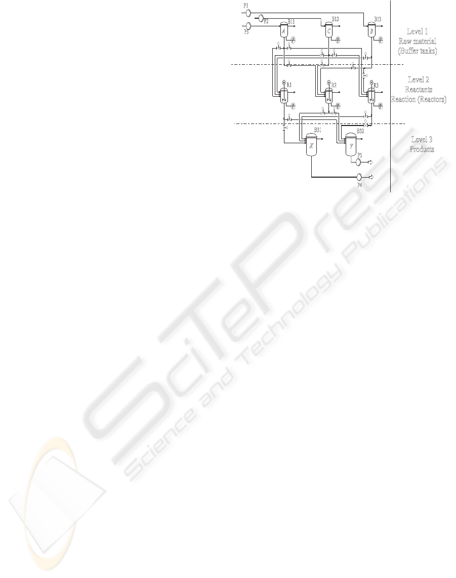
presented by (Bauer et al., 2000) is considered. The
case study is a multi-product chemical batch plant
with 3 stages in which two end-products, X and Y,
are produced from three raw materials, A, B and C.
The production process considered is: one batch of
material A and C each reacts to produce one batch of
product X; similarly one batch of B and C reacts to
produce one batch of product Y. The plant executing
the production process is shown in Figure 5.
The first stage consists of three buffer tanks B11,
B12 and B13 that store the raw materials A, C and
B. The second stage consists of three reactors R1, R2
and R3. Each reactor may be filled from each raw
material buffer tank in the first stage; implying that it
is possible to produce either product X or Y in each
reactor. After processing the materials a reactor may
B11
R1
R3
R2
M
M
M
B13
B31
B32
P1
P3
LIS
LIS
LIS
LIS
LIS
LIS
13
11
21
22
23
12
B12
P2
Level2
Reactants
Reaction(Reactors)
Level3
Products
Level1
Rawmaterial
(Buffertanks)
P5
P4
A
C
B
X
Y
Figure 5: The structure of the example process.
contain one batch of the product (resulting from two
batches of raw material). The third stage consists of
two buffer tanks B31 and B32 which are used to store
the end-products X and Y. Each of the tanks has a
maximum capacity to store three batches of the prod-
uct. The proposed scheduling problem is to derive
production schedules to produce 2 batches of the end-
products with a minimum makespan. After being pro-
cessed by the reactors the materials must be drained
into the buffer tanks in the third stage immediately.
RTN description of the problem considered is
shown in Figure 6. Materials A, C and B are rep-
resented as S
1
,S
2
and S
3
. The tasks T
1
,T
2
and T
3
represents the task of pumping materials A, C and B
into buffer tanks B11, B12 and B13, respectively. The
tasks T
4
,T
6
and T
8
represent the step of draining one
batch of A from B11 into the reactors R1, R2 and R3.
Similarly, tasks T
11
, T
13
and T
15
represent draining of
material B from B13 into the reactors. The tasks T
5
,
T
7
and T
9
represent mixing one batch of C from B12
with one batch of A, already present in R1, R2 and R3
in order to produce X. The tasks T
10
,T
12
and T
14
rep-
resent similar actions for producing one batch of Y.
The tasks T
16
,T
17
and T
18
represent the step of drain-
ing one batch of X from R1, R2 and R3, respectively,
into the buffer tank B31. Tasks T
19
,T
20
and T
21
rep-
resent draining one batch of Y from R1, R2 and R3
into tank B32. The tasks T
22
and T
23
represent drain-
ing of two batches of X from B31 and two batches
of Y from B32 to the product storage, respectively.
The constraint on the waiting time is expressed by the
places P
2
, P
4
, P
6
, P
8
, P
10
and P
12
. The places P
1
, P
3
,
P
5
, P
7
, P
9
and P
11
are established to ensure that mate-
rial C is drained into the reactors only after either A
or B has been drained.
ICINCO 2007 - International Conference on Informatics in Control, Automation and Robotics
146
R
1
S
1
0.5
T
1
[0,0]
[0,0]
[0,0]
[0,0]
[0,0]
[0,0]
[0,0]
[0,0]
[0,0]
[0,0]
[0,0]
[0,0]
S
4
S
2
S
5
S
3
S
6
S
12
S
11
S
10
S
9
S
8
S
7
S
13
S
15
S
16
S
14
T
4
T
5
T
6
T
16
T
17
T
22
T
18
T
7
T
8
T
9
T
10
T
11
T
12
T
13
T
15
T
14
T
2
T
3
T
19
T
20
T
23
T
21
0.5
0.5 0.5
0.5 0.5
0.5 0.5 0.5 0.5 0.5
0.5
R
4
R
5
R
2
R
6
R
4
R
3
R
5
R
6
R
7
R
9
R
8
R
10
P
1
P
2
P
3
P
4
P
5
P
6
P
7
P
8
P
9
P
10
P
11
P
12
Figure 6: The RTN of the example process.
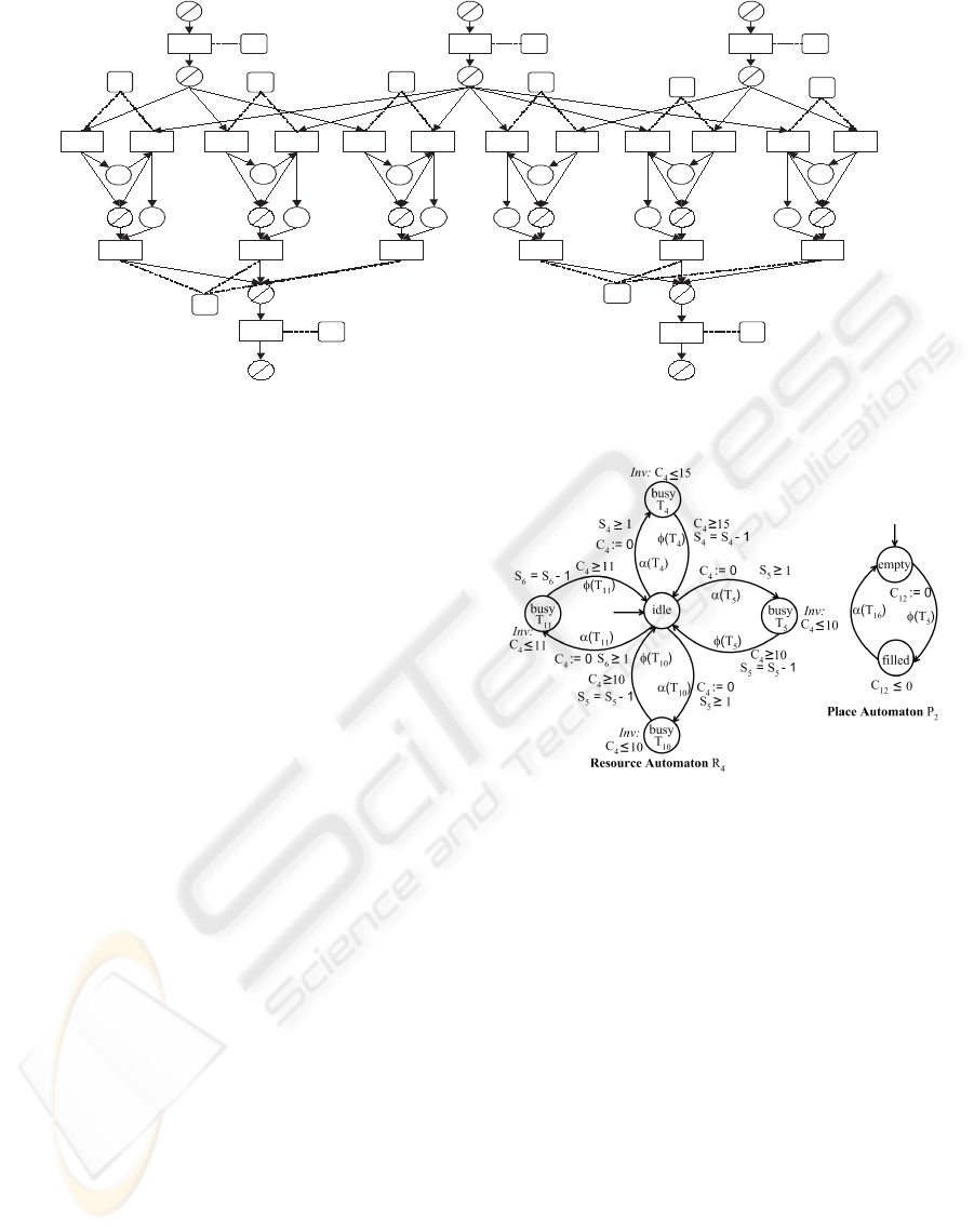
5.1 TA Model
The TA model consists of 10 resource automata to
model the individual resources. The places are mod-
eled as separate automata. The resource automata and
the place automata have one clock each to measure the
task durations and time interval for storage. An addi-
tional global clock which is never reset is included in
the model to measure the makespan. The resource au-
tomaton for resource R
4
and the place automaton P
2
are shown in Figure 7. The automaton R
4
has one idle
location and four busy locations indicating the exe-
cution of either of the tasks T
4
or T
5
or T
10
or T
11
.
Tasks T
4
and T
11
process one batch of material S
4
and
S
6
with task duration of 15 and 11 units. The tim-
ing constraint between task T
5
and task T
16
is mod-
eled by the place automaton P
2
on the right side. Task
T
5
after finishing its process in R
4
produces a token
in the place P
1
by taking the synchronized transitions
in R
5
and P
2
with the label φ
5
. The clock C
12
is re-
set and forces P
2
to leave the location filled without
waiting. This happens by starting task T
16
and by tak-
ing the synchronized transitions with label α
16
in R
7
and P
2
. An automatic translation from the RTN to the
TA model was performed by the tool TAOPT (Panek
et al., 2005).
5.2 Computational Experiments
The scheduling problem presented in the example
process was solved by a Xeon machine with a CPU
speed of 3.06 GHz, 2.0 GB of memory and a linux op-
erating system. For the cost optimal symbolic reacha-
bility analysis, the software tool TAOPT (Panek et al.,
2005) which supports different state space reduction
techniques as discussed above: immediate traces,
Figure 7: Structure of the resource and place automaton.
(strict) non-lazy runs and sleep-set method was used.
A combination of the depth-first and best-first strategy
was used for exploring the graph. Among the nodes
in the waiting list, the node with the maximum depth
is given a higher priority, among the nodes with the
same depth, priority is given to the node with a mini-
mum cost. If two or more nodes have the same depth
and cost, one of them is chosen randomly.
The Table 1 shows the results obtained by re-
stricting the search to only immediate traces repre-
sented as None and with other state space reduction
techniques: ordinary non-lazy runs (NL
ordinary
), strict
non-lazy runs and strict sleep-set method (SSM
strict
).
For all tests the complete reachability graph was ex-
plored. The second column that represents the total
time needed to compute the reachability graph and the
total number of nodes explored in the the third column
reveal that the strict sleep-set method reduces the state
space and computational effort considerably. On the
other hand it prunes the optimal solutions. The fourth
column represents the time taken in CPU seconds to
SCHEDULING OF MULTI-PRODUCT BATCH PLANTS USING REACHABILITY ANALYSIS OF TIMED
AUTOMATA MODELS
147

Table 1: Computational results.
First solution Best solution
Reduction technique Total time Total nodes time nodes C
max
C
max
None 58.832 493167 0.032 1875 100 98
NL
ordinary
2.104 37483 0.048 2157 98 98
SSM
strict
0.476 13374 0.120 6492 131 128
SSM + NL
ordinary
1.084 28583 0.040 681 102 98
compute the first feasible solution when different re-
duction techniques were used. The test with nor-
mal sleep set method which compares and removes
only time persistent pairs of transitions in combina-
tion with ordinary non-lazy runs was performed. This
is represented as SSM + NL
ordinary
in the table 1. The
combination of SSM + NL
ordinary
found the optimal
solution. This is due to the fact that only time per-
sistent transitions were pruned. No solutions could
be found for the strict non-laziness setting when ap-
plied alone or in combination with the strict sleep-set
method and the normal sleep-set method. It should
be noted that the reduction techniques ordinary non-
lazy runs and the normal sleep-set method are the
only combinations which theoretically guaranty that
the optimal solution is not pruned. The strict sleep set
method in general should only be used as a heuristic.
6 CONCLUSION
A new and a straightforward approach to model
scheduling problems in multi-product batch plants
and to derive production schedules based on symbolic
reachability analysis of TA has been introduced. The
experimental results show that the method can solve
scheduling problems in process industries efficiently
within a limited computation time. The main aspect
to be considered is the time required by the TA ap-
proach to specify and formulate the scheduling prob-
lem. It is relatively easy when compared to formulat-
ing it as MILP which are usually cumbersome. The
efficiency of the approach to derive solutions with re-
duced computational effort have been achieved with
different search space reduction techniques.
Future work on the TA based approach will focus
on online scheduling problems in which the arrival
time of jobs is not known in advance and subject to
random perturbations.
ACKNOWLEDGEMENTS
The authors gratefully acknowledge the financial sup-
port by the Graduate School of Production Engineer-
ing and Logistics at the University of Dortmund.
REFERENCES
Abdeddaim, Y. and Maler, O. (2001). Job-shop scheduling
using timed automata. Computer Aided Verification
(CAV), Springer, pages 478–492.
Alur, R. and Dill, D. (1994). A theory of timed automata.
Theor. Comp.Science, 126(2):183–235.
Barthomieu, B. and Diaz, M. (1991). Modeling and
verification of time dependent systems using timed
petri nets. IEEE Transactions Software Engineering,
126(2):259–273.
Bauer, N., Kowalewski, S., Sand, G., and Loehl, T. (2000).
A case study: Multi product batch plant for the
demonstration of scheduling and control problems.
In ADPM2000 Conference Proceedings-Hybrid Dy-
namic Systems, pages 383–388. Shaker.
Behrmann, G., Fehnker, A., Hune, T., Peterson, P., Larsen,
K., and Romjin, K. (2001). Efficient guiding to-
wards cost-optimality in UPPAAL. In Proceedings
TACAS’01, pages 174–188.
Godefroid, P. (1991). Using partial orders to improve auto-
matic verification methods. In Proc. 2nd Workshop on
Computer Aided Verification, 531 of LNCS:176–185.
Kallrath, J. (2002). Planning and scheduling in the process
industry. OR Spectrum, 24:219–250.
Panek, S., Engell, S., and Lessner, C. (2005). Scheduling
of a pipeless multi-product batch plant using mixed-
integer programming combined with heuristics. In Eu-
ropean Symposium on Computer Aided Process Engi-
neering, ESCAPE 15, pages 1033–1038.
Panek, S., Engell, S., and Stursberg, O. (2006). Efficient
synthesis of production schedules by optimization of
timed automata. Control Engineering Practice, pages
149–156.
Panek, S., Engell, S., Subbiah, S., and Stursberg, O. (2007).
Scheduling of multi-product batch plants based upon
timed automata models. Submitted to Comp. Chem.
Eng.
Pantelides, C. (1994). Unified frameworks for optimal pro-
cess planning and scheduling. In Proceedings 2nd
conference Foundations of Computer Aided Process
Operations, pages 253–274.
ICINCO 2007 - International Conference on Informatics in Control, Automation and Robotics
148
