
DECENTRALIZED APPROACH FOR FAULT DIAGNOSIS OF
DISCRETE EVENT SYSTEMS
Moamar Sayed Mouchaweh
a
, Alexandre Philippot
b
and Véronique Carré-Ménétrier
a
a
Université de Reims, CReSTIC, Moulin de la Housse 51687 Reims - France
b
LURPA, ENS de Cachan, 61 avenue du Président Wilson, 94235 Cachan Cedex, France
Keywords: Fault diagnosis, Discrete Event Systems, Decentralized diagnosis, Co-diagnosability notion.
Abstract: This paper proposes a decentralized approach to realize the diagnosis of Discrete Event Systems (DES).
This approach is based on a set of local diagnosers, each one of them diagnoses faults entailing the violation
of the local desired behavior. These local diagnosers infer the fault’s occurrence using event sequences, time
delays between correlated events and state conditions, characterized by sensors readings and commands
issued by the controller. An adapted codiagnosability notion is formally defined in order to ensure that the
set of local diagnosers is able to diagnose all faults entailing the violation of the global desired behavior. An
example is used to illustrate the proposed approach.
1 INTRODUCTION
Manufacturing systems are too large to perform a
centralized diagnosis. Moreover, they are
informationally and geographically decentralized.
Thus a diagnosis module with a decentralized
structure is the most adapted one for this kind of
systems. However, the challenge of decentralized
diagnosis methods is to perform local diagnosis
equivalent to the centralized one. Indeed, the partial
observation of the system may lead to an ambiguity
of the final diagnosis decision. Examples of DES
decentralized diagnosis methods can be found in
(Debouk, 2000), (Pandalai, 2000), (Qiu, 2005), and
the references therein.
Failure diagnosis in DES requires that once a
failure is occurred, it must be detected and isolated
within a bounded delay or number of events. This
property is verified using a notion of diagnosability.
This notion can be formalized differently according
to whether the fault is modelled as the execution of
certain faulty events, event-based notion, or as the
consequence of reaching at certain faulty states,
state-based notion. In (Sampath, 1994), an event-
based diagnosability notion is defined. The system
model is based on a finite-state automaton. This
notion defines a diagnoser that uses the history of
events to detect the occurrence of a failure.
Consequently, a system is diagnosable if and only if
any pair of faulty/non-faulty behaviors can be
distinguished by their projections to observable
behaviors. The event-based diagnoser can diagnose
actuator and sensor permanent and intermittent
failures. However, the diagnoser and the system
model must be initiated at the same time to allow the
system model and diagnoser to response
simultaneously to events. This initialization is hard
to obtain in manufacturing systems since their initial
state may not be known. To enhance the
diagnosability, the above framework is extended to
dense-time automata (Tripakis, 2002). This
extension is useful since it permits to model plants
with timed behavior.
In (Pandalai, 2000), an event-based approach is
proposed to monitor manufacturing systems. In this
approach, the timed sequence events, generated by
the DES, is compared with a set of specifications of
normal functioning called templates. These
templates are based on the notion of expected event
sequencing and timing relationships. They are
suitable for modelling processes in which both
single-instance and multiple-instance behaviors are
exhibited concurrently. However, these templates do
not allow the analysis of diagnosability properties,
which are based on a diagnosability notion.
To find a remedy to the initialization problem, a
state-based diagnosability notion is proposed in (Lin,
1994), (Zad, 2003). In this notion, since the system
states describe the conditions of its components,
124
Sayed Mouchaweh M., Philippot A. and Carré-Ménétrier V. (2007).
DECENTRALIZED APPROACH FOR FAULT DIAGNOSIS OF DISCRETE EVENT SYSTEMS.
In Proceedings of the Fourth International Conference on Informatics in Control, Automation and Robotics, pages 124-129
DOI: 10.5220/0001627301240129
Copyright
c
SciTePress

diagnosing a fault can be seen as the identification in
which state or set of states the system belongs to.
However, the diagnosis is limited to the case of
actuator faults. While manufacturing systems use
many sensors entailing the necessity of diagnosing
also their faults.
This paper presents a decentralized diagnosis
approach to perform the diagnosis of manufacturing
systems. The paper is structured as follows. Firstly,
the different steps of the proposed approach
necessary to construct the local diagnosers are
detailed. Secondly, a timed-event-based
diagnosability notion is presented. Then, in order to
verify the codiagnosability property of local
diagnosers, this notion is extended to the
codiagnosability notion. Finally, a simple example is
used to illustrate the proposed approach.
2 DECENTRALIZED DIAGNOSIS
APPROACH
2.1 System Boolean Models
We use Boolean DES (BDES) modelling, introduced
in (Wang, 2000), to model the equipments (sensors
and actuators) behavior of the system. The system
model G consists of n local models: G
1
,…, G
n
, each
one owns its local observable events responsible of a
restricted area of the process. G
i
= (Σ, Q, Y,
δ
, h, q
0
)
is represented as Moore automaton and L = L(G)
denotes its corresponding prefixed closed language.
Σ is a set of finite observable and unobservable
events. Q is the set of states, Y is the output space,
δ
:
Σ
*
x Q
→
Q is the state transition function and Σ
*
is
the set of all event sequences of the language L(G).
δ
(
σ
, q) provides the set of possible next states if
σ
occurs at q. h: Q
→
Y is the output function and
h(q) is the observed output at q.
0
q is the initial
state.
Let Σ
Π
= {
Π
F1
,
Π
F2
,…,
Π
Fr
} be the set of fault
partitions. Each fault partition,
Π
Fj
, j ∈ {1, 2,…, r},
corresponds to some kind of faults in an equipment
element (sensor or actuator). We assume at most one
fault may occur at a time. These faults must be
considered when BDES models.
In (Balemi, 1993), Balemi et al. defined
controllable events Σ
c
⊆ Σ as controller’s outputs
sent to actuators, and uncontrollable events Σ
u
⊆ Σ
as the controller’s inputs coming from sensors. (Σ
o
=
Σ
c
∪ Σ
u
) ⊂ Σ is the set of observable events. The
unobservable events are failure events or other
events which cause changes not recorded by sensors.
Let G
i
and its corresponding prefixed closed
language, L
i
= L(G
i
), be the local model of the
restricted area of the system observed by this model.
G
i
= (Σ
i
, Q
i
, Y
i
,
δ
i
, h
i
, q
0
i
) is represented as Moore
automaton. Σ
0
i
= Σ
c
i
∪ Σ
u
i
is the set of local
observable events by G
i
and Σ
0
i
⊂ Σ
0
. The other
notations have the usual definition but for the
restricted area observed by G
i
.
G observes the system by one global projection
function or mask, P
L
: Σ
*
∪ {
ε
} → Σ
0
*
, where Σ
0
*
is
the set of all observable event sequences observed
by G. The inverse projection function is defined as:
P
L
-1
(u) = {s ∈ L: P
L
(s) = u}. Similarly, a local
projection function can be defined for each local
model G
i
as: P
i
: Σ
i*
∪ {
ε
} → Σ
0
i*
.
Each state q
j
of G is represented by an output
vector h
j
considered as a Boolean vector whose
components are Boolean variables. Let d denote the
number of state variables of G, the output vector h
j
of each state q
j
can be defined as:
∀q
j
∈ Q, h(q
j
) = h
j
= (h
j1
,…, h
jp
,…, h
jd
), h
jp
∈ {0, 1},
1 ≤ j ≤ 2
d
, h
j
∈ Y ⊆
d
I
Β
A transition from one state to another is defined
as a change of a state variable from 0 to 1, or from 1
to 0. Thus each transition produces an event
α
characterized by either rising,
α
= ↑h
jp
, or falling,
α
=
↓h
jp
, edges where p ∈ {1, 2,…, d}.
To describe the effect of the occurrence of an
event
α
∈ Σ
0
, a displacement vector E
α
= (e
α
1
,…,
e
α
p
,…, e
α
d)
is used. If e
α
p
= 1, then the value of p
th
state variable h
jp
will be set or reset when
α
occurs.
While if e
α
p
= 0, the value of p
th
state variable h
jp
will remain unchanged:
α
α
δ
Σ
α
Ehh)q,(q,,Qq,q
ijijoji
⊕=⇒
=
∈
∀
∈
∀
(1)
The set of all the displacement vectors of all the
events provides the displacement matrix E. For each
event
α
∈ Σ
0
, an enablement condition, en
α
(q
i
) ∈ {0,
1}, is defined in order to indicate if the event
α
can
occur at the state q
i
, en
α
(q
i
) = 1, or not:
))q(en.E(hh)q,(q,,Qq,q
iijijoji
αα
α
δ
Σ
α
⊕=⇒
=
∈
∀
∈
∀
(2)
2.2 Constrained-System Boolean Model
Let S = (Σ, Q
S
, Y,
δ
S
, h, q
0
) denote the constrained-
system model, characterized as Moore automaton. It
defines the global desired behavior of the system
and it is represented by the prefixed closed
specification language K = L(S) ⊆ L(G). S can be
obtained using different algorithms from the
literature as the ones developed in (Philippot, 2005),
DECENTRALIZED APPROACH FOR FAULT DIAGNOSIS OF DISCRETE EVENT SYSTEMS
125

(Ramadge, 1987) and the references therein. To
obtain the transition function
δ
S
, the enablement
conditions for all the system events at each state
must satisfy all the specifications K, representing the
desired behavior:
))q(en.E(hh,)q(en
)q,(q,Qq,q,
iiji
iSjSji
ααα
α
δ
Σ
α
⊕==
⇒=∈∀∈∀
1
0
(3)
Each local model G
i
has a local constrained
model S
i
, which is a part of the global constrained
model S. S
i
is represented by the specification
language K
i
= L(S
i
), which is included in K. S
i
is
Moore automaton: S
i
= (Σ
i
, Q
i
S
, Y
i
,
δ
i
S
, h
i
, q
i
0
) and Q
i
S
⊂ Q
i
. All these notations have the usual definition
but for the local constrained-system model S
i
.
2.3 Codiagnosability Notion
2.3.1 Basic Definitions
Let
Ψ
Fj
define the set of all the event sequences
ending by a fault belonging to the fault partition
Π
Fj
.
Thus
)(
j
F
r
jF
Ψ
Ψ
1=
= ∪
denotes the set of all the event
sequences ending by a fault belonging to one of fault
partitions of Σ
Π
. Consequently
Ψ
F
⊆ (L - K), i.e., all
the faulty sequences are considered as violation of
the specification language K. The set of faulty states
is defined as S
F
:
)S(
j
F
r
j 1=
∪
where S
Fj
is the set of
states reached by the occurrence of a fault of F
j
. Let
H
Fj
denote the set of all state output vectors of the
faulty states belonging to S
Fj
. Then the output
partition H
Fj
can be defined as:
∀q’ ∈ S
Fj
, h’ = h(q’) ⇒ h’ ∈ H
Fj
.
The set of fault labels Λ
F
= {F
1
, F
2
,..., F
r
}
indicates the occurrence of a fault belonging to one
of the fault partitions Σ
Π
. By adding the normal label
N, we can obtain the set Λ of all the labels used by
the diagnoser. We define the label function l: Q → Δ
to indicate the functional status of the system when
it reaches a state q ∈ Q. Δ is the set of all possible
subsets of the diagnoser labels:
{}{ }{ } { }
{
}{ }
{}{}{ }{ }
.
F,...,F,N,...,F,F,N,F,N,...,F,N
,F,...,F,F,F,F,F,...,F,F,N
rr
rr
⎭
⎬
⎫
⎩
⎨
⎧
=
1211
212121
Δ
Similarly, we can define Δ
F
as the set of all the
subsets of fault labels.
2.3.2 Events Timing Delays Modelling
The majority of sensors and actuators in
manufacturing systems produce constrained events
since state’s changes are usually effected by a
predictable flow of materials (Pandalai, 2000).
Therefore, we define a set of expected consequents
EC
β
for each controllable event,
β
∈
Σ
c
, in order to
predict uncontrollable but observable consequent
events within pre-defined time periods. This EC
β
describes the next events that should occur and the
relative time periods in which they are expected.
These pre-defined time periods are determined
by experts according to the system dynamic and to
the desired behavior. If u =
k
α
α
βα
...
21
is an
observable event sequence starting by a controllable
event
β
, and ending by the observable event
sequence
*
21
...
uok
Σ⊂
ααα
, then the set of expected
consequents
)(uEC
β
is created when the event
β
occurs.
)(uEC
β
has the following form: )(uEC
β
=
{
}
β
α
β
α
β
α
β
α
ki
C,...,C,...,C,C
21
.
β
α
i
C
is a consequent expected
after the enablement of the controllable event
β
and
it is defined as follows:
{
}
),],[,(,,
max
min
i
iq
ii
i
i
lttqC ij
ααα
α
β
α
α
α
α
=
. It means that when
j
α
occurs, the event
i
α
should happen at the state
i
q
α
and within the interval [
i
t
α
min
,
i
max
t
α
]. If it is the case
then the expected consequent is satisfied. If the
event
i
α
has occurred before
i
min
t
α
or after
i
max
t
α
then
the expected consequent is not satisfied and it
provides the fault label
F
q
i
i
l
Δ
α
α
∈ , as the cause of
this non-satisfaction. This set of expected
consequent
)(uEC
β
is evaluated by a function
)(uEF
β
. )(uEF
β
is equal to 1 if one of its expected
consequents is not satisfied while it is equal to zero
if all its expected consequents are satisfied.
2.3.3 Codiagnosability Notion Formulation
If a system composed of n local diagnosers with a
global closed prefixed language L, a global closed
prefixed specification language K, a global
projection function P, and a predefined set of fault
partitions, Σ
Π
= {
Π
F1
,
Π
F2
,…,
Π
Fr
}, is diagnosable
using a central diagnoser. Then this system is F-
codiagnosable according to the projection functions,
P
i
: i = 1 … n, if and only if :
{
}
{}
{}
{}
jz
i
z
F
i
F
ii
FF
FlstPEFm,...,,z
Hhqhh,q,uq,Qq
)KL(u
KLstPPu,kt,n,...,,i
,KLst,r,...,,j,f,INk
j
j
jj
==⇒∈∃
∈
′
⇒
′
=
′
=
′
∈∀
∩−∈⇒
⎥
⎥
⎦
⎤
−∩∈∀≥∈∃
∩−∈∀∈∈∀∈∃
−
and1))((21
)()(
)()(21
)(21
1
δ
Ψ
ΨΠ
(4)
The satisfaction of (4) means that the occurrence
of a fault of the type F
j
is diagnosable by at least one
local diagnoser D
i
, using the event-based, state-
based or timed local models. Indeed if the faulty
event sequence s, ending by a fault of the type F
j
, is
ICINCO 2007 - International Conference on Informatics in Control, Automation and Robotics
126
distinguishable by the central diagnoser D after the
execution of k = |t| transitions, where t is a
continuation of s. If u is any other event sequence
belonging to (L – K) and producing the same
observable event sequence as st, P
i
(u) = P
i
(st),
according to the local diagnoser D
i
. Then the system
is F-codiagnosable if and only if:
• u contains in it a fault of the type F
j
, (event-
based model),
• u transits D
i
to a state characterized by an output
vector belonging to the output partition H
Fj
,
(state-based model),
• There is at least one expected consequent,
defining a temporal constraint between the
occurrence of the observable events P
i
(st) by the
diagnoser D
i
, not satisfied. This expected
consequent is evaluated by an expected function
which provides a fault label l = {F
j
} as the cause
of this non-satisfaction, (timed-model).
2.3.4 Codiagnosability Checking
The set of local diagnosers are able to diagnose any
fault belonging to one of the fault partitions of F and
within a finite delay, if:
{}
1)(,,...,2,1,, =⇒∈∃∈∀∈∈∀ qenQqniKL
i
ρ
ρρ
(5)
{} {}
{}
jq
i
q
i
F
Fl(PEFqenQq
,n,...,,i,,r,...,,j,KL,L
j
===⇒∈∃
∈∃≠∩∈∀−∈∈∀
and)1))(or0)((
2121
ρ
ϕψρρρ
ρ
(6)
Nk ∈≤
ρ
(7)
(5) means that all the enablement conditions of
all the local diagnosers must be satisfied for any
event of a sequence belonging to the global desired
behavior. Thus this condition ensures that no
conflict can occur between local diagnosers for the
enablement of events at any state of the desired
behavior. The satisfaction of (6) ensures that any
event sequence violating the global desired behavior,
due to the occurrence of a fault of the type F
j
, must
be diagnosed by at least one local diagnoser D
i
when
it reaches the state q. This detection and isolation are
based on the non-satisfaction either of the
enablement condition of the latest event in the event
sequence
ρ
or of its expected function. In the both
cases, this non-satisfaction should provide the fault
label F
j
. Finally (7) guarantees that this diagnosis
decision will be realized in a finite delay equal to the
cardinality of the event sequence
ρ
.
3 ILLUSTRATION EXAMPLE
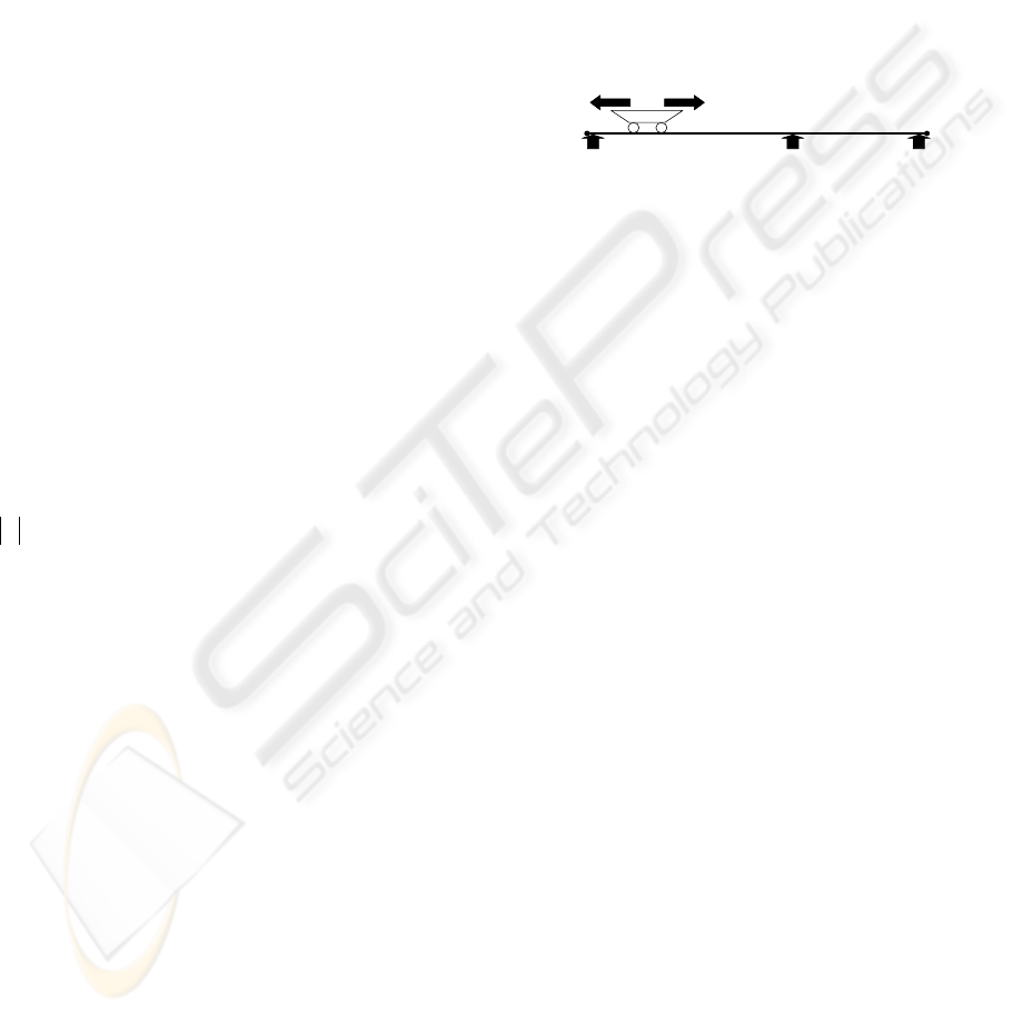
3.1 Example Presentation
We monitor a wagon with an electric actuator with
two senses of movement: right and left, obtained by
two commands, R for the movement right and L for
the movement left. Three sensors a, b and c are used
to indicate the wagon location in, respectively, A, B
or C, as it is illustrated in Figure 1. We have chosen
this simple example for easy understanding. The
same reasoning can be followed for the application
of the approach on more complex examples.
L R
a b
AB A-B
c
C B-C
Figure 1: Illustration example.
The following hypotheses must hold:
• The wagon inertia is null,
• Actuator does not fail during operation, i.e., if it
does fail, the fault is at the start of operation,
• There are no ambiguity or indecision cases
between the local diagnosers.
The system is modelled with two sub models: G
1
and G
2
. Their local observable events are
respectively: Σ
0
1
= {↑R, ↓R, ↑L, ↓L, ↑a, ↓a, ↑b, ↓b}
and Σ
0
2
= {↑R, ↓R, ↑L, ↓L, ↑b, ↓b, ↑c, ↓c}. We use
five Boolean state variables a, b, c, R and L to
describe the overall wagon behavior G. a, b and c
are true when the wagon is located respectively in A,
B or C.
Each local model consists of two components:
the wagon motor behavior and the change of the
wagon location measured by the sensors a and b for
G
1
, and b and c for G
2
. The set of fault partitions to
be diagnosed is F = {F
1
, F
2
, F
3
, F
4
}. F
1
, F
2
, F
3
and
F
4
indicate, respectively, sensor a, sensor b, sensor c
and wagon motor stuck-on or stuck-off.
3.2 Constrained System Models
The constrained-system model S for the wagon
example is depicted in Figure 2 and is provided by
the user. S
1
and S
2
represent the local desired
behaviors for the two sub models G
1
and G
2
according to their set of local observable events.
In BDES modelling, this desired behavior can be
described using two tables; the first one explains the
enablement conditions for the occurrence of each
event and the second one is the displacement matrix
for the estimation of the state output vector of each
DECENTRALIZED APPROACH FOR FAULT DIAGNOSIS OF DISCRETE EVENT SYSTEMS
127
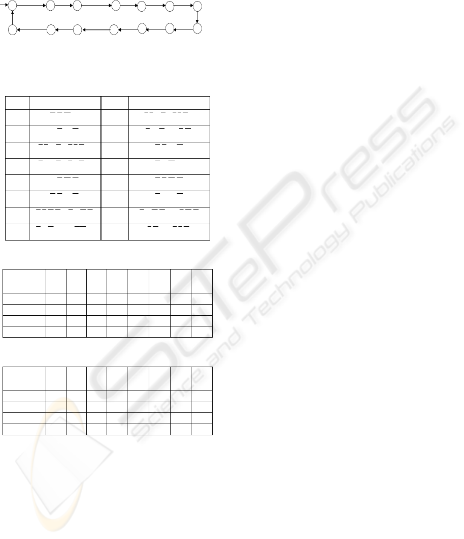
next state. These tables are shown respectively in
Table 1, Table 2 and Table 3 for S
1
and S
2
.
1 2
↑ R
14 13
↑a
3 4
↑b
12 11
↑ L
↓
a
↓
b
↓
L
h
: a
b
c
R
L
10000 10010 0001
0
01010
01000 10001 00001 01001
5 6
9 8
↑b
7
↑c
10
↑
L
↓
b
↓
c
↓
L
↓
R
0001
0
00110 00100
001010000101001
Figure 2: Global constrained-system model S .
Table 1: The enablement conditions for S
1
and S
2
.
σ: S
1
en
σ
σ: S
2
en
σ
↑a
LRba ...
↑b
LRcbLRcb ...... +
↓a
LRba ...
↓b
LRcbLRcb ...... +
↑b
LRbaLRba ...... +
↑c
LRcb ...
↓b
LRbaLRba ...... +
↓c
LRcb ...
↑R
LRba ...
↑R
LRcb ...
↓R
LRba ...
↓R
LRcb ...
↑L
LRbaLRba ...... +
↑L
LRcbLRcb ...... +
↓L
LRbaLRba ...... +
↓L
LRcbLRcb ...... +
Table 2: The displacement matrix E
1
for S
1
.
State
variable
↑a ↓a ↑b ↓b ↑R ↓R ↑L ↓L
a 1 1 0 0 0 0 0 0
b 0 0 1 1 0 0 0 0
R 0 0 0 0 1 1 0 0
L 0 0 0 0 0 0 1 1
Table 3: The displacement matrix E
2
for S
2
.
State
variable
↑b ↓b ↑c ↓c ↑R ↓R ↑L ↓L
b 1 1 0 0 0 0 0 0
c 0 0 1 1 0 0 0 0
R 0 0 0 0 1 1 0 0
L 0 0 0 0 0 0 1 1
3.3 Expected Consequents Definition
Two expected consequents are defined for G, one for
each command enablement: EC
↑R
, EC
↑L
. The
enablement of R, entails the events
↓a, ↑b, ↓b, and ↑c
to occur respectively at the states q
2
, q
3
, q
4
, and q
5
.
↓a is expected to occur within the time period [1,2],
after the enablement of R,
↑b within the time period
[3,5] after the occurrence of
↓a, ↓b inside the
interval [1,2], and
↑c inside [3,5] according to the
system dynamic. If
↓a does not occur at q
2
then the
wagon motor has not responded. Thus the non-
satisfaction of the corresponding expected
consequent at this state indicates the occurrence of a
fault belonging to
Π
F4
. If ↓a has occurred, then S
will transit to the state q
3
. If ↑b has not occurred,
then the non-satisfaction of the corresponding
expected consequent provides the label l = {F
2
} to
indicate that the sensor b is faulty, stuck-off, since
the wagon has responded. Similarly the non
occurrence of
↓b at q
4
indicates that the sensor b is
stuck-on. Consequently EC
↑R
can be written:
R
EC
↑
=
{
}{ }
{}{}
⎪
⎭
⎪
⎬
⎫
⎪
⎩
⎪
⎨
⎧
↑↓↓↑
↑↓↓↑
)F],,[,q(,c,b,)F],,[,q(,b,b
,)F],,[,q(,b,a,)F],,[,q(,a,R
3524
2342
5321
5321
.
Similarly the expected consequent for the
enablement of the command L can be written:
L
EC
↑
=
{
}{ }
{}{}
⎪
⎭
⎪
⎬
⎫
⎪
⎩
⎪
⎨
⎧
↑↓↑↓
↓↑↓↑
)]53[(]53[
)]21[()]21[(
29113
41248
F,,,q,b,c,F,,,q(,a,b
,F,,,q,b,L,F,,,q,c,L
.
3.4 Local Diagnosers Construction
Two local diagnosers D
1
and D
2
are constructed for
the sub models S
1
and S
2
. Each local diagnoser
contains, besides the states of the local desired
behavior model, all the faulty states that can be
reached by the occurrence of a fault belonging to
one of the fault partitions. Each one of these faulty
states is reached due to the non-satisfaction either of
the enablement condition of an event or of an
expected consequent. This makes the diagnoser
declaring a fault. The diagnosers D
1
and D
2
are
depicted respectively in Figure 3 and Figure 4. Each
diagnoser state is determined by testing whether the
enablement condition, or the expected consequent, is
satisfied (the next state is a desire one) or not (the
next state is faulty). The fault labels are calculated
by determining the reason of the non-satisfaction.
The diagnoser can be initiated at any state
distinguished by its output vector, i.e., the states
with the dotted entrant arrows. If the diagnoser is
initiated at any state distinguished by an event, the
diagnoser cannot diagnose a past occurrence of a
fault. As an example, the faulty states reached by an
unsatisfied expected consequent cannot be
distinguished from the ones of the desired behavior
if the diagnoser was initiated at one of these states.
The system is F-codiagnosable if it satisfies the
conditions (5), (6) and (7). The condition (5) is
satisfied since the two diagnosers authorize both the
events observable by them:
,q∀ 0.
21
≠
↑↑ bb
enen and
0.
21
≠
↓↓ bb
enen
. The condition (6) is also verified
since the local diagnosers can diagnose with
certainty the occurrence of a fault belonging to one
of the fault partitions of Σ
Π
.
ICINCO 2007 - International Conference on Informatics in Control, Automation and Robotics
128

D
1
diagnoses with certainty the faults belonging
to one of
Π
F1
,
Π
F2
and
Π
F4
while D
2
diagnoses with
certainty the faults belonging to one of
Π
F2
,
Π
F3
and
Π
F4
. Finally (7) holds since the delay required to
diagnose a fault belonging to one of the fault
partitions, in the worst case and for any one of the
two diagnosers, is finite and equal to 6 events. If we
consider the non-satisfaction of an expected
consequent as an event then starting from any
diagnoser state of the desired behavior, the longest
event sequence required to decide the occurrence of
a fault is maximally equal to 6. As an example,
starting from the state 7 of D
1
, the detection of the
occurrence of a fault belonging to one of
Π
F1
,
Π
F2
or
Π
F4
requires, respectively, 6 events (state 21), 5
events (state 20) and 5 events (state 19). Thus, the
system is F-codiagnosable.
1110
15
F
1
↑
R
↓
a
↑
b
↓
b
↓
R
↑
b
0010
17
F
2
1000
1
N,F
1
,F
2
,F
4
1010
2
N,F
1
,F
2
,F
4
0010
3
N,F
1
,F
2
0110
4
N,F
1
,F
2
0010
5
N,F
1
,F
2
0000
7
N,F
1
,F
2
,F
4
1010
16
F
4
abRL
q
l
D
1
0110
18
F
2
1101
20
F
2
↓
b
↑
a
↑
L
0001
21
F
1
0001
8
N,F
1
,F
2
,F
4
0101
10
N,F
1
,F
2
0100
11
N,F
1
,F
2
,F
4
0101
12
N,F
1
,F
2
,F
4
0001
13
N,F
1
,F
2
1001
14
N,F
1
,F
2
↓
L
↑
b
↑
L
↓
L
1010
19
F
4
↑
a
EF
↑
L
(
↓
b
↑
a
)=1
EF
↑
L
(
↑
L
↓
b)=1
EF
↑
R
(
↓
a
↑
b)=1
EF
↑ R
(
↑
R
↓
a)=1
EF
↑ R
(
↓
b
↑
b)=1
Figure 3: Local event-state-based diagnoser, D.
1
1110
22
F
2
0001
27
F
2
↑ R
↑ b ↓ b ↑ c ↓ R
↑ L ↓ b
↑ L
↑c
1010
23
F
2
0000
1
N,F
2
,F
3
,F
4
0010
3
N,F
2
,F
3
,F
4
1010
4
N,F
2
,F
3
,F
4
0010
5
N,F
2
,F
3
0110
6
N,F
2
,F
3
0100
7
N,F
2
,F
3
,F
4
0101
8
N,F
2
,F
3
,F
4
0001
9
N,F
2
,F
3
1110
26
F
3
bcRL
q
l
D
2
1001
10
N,F
2
,F
3
,F
4
1000
11
N,F
2
,F
3
,F
4
1001
12
N,F
2
,F
3
0001
13
N,F
2
,F
3
↑ b ↓ c
0010
24
F
3
↓ L
↓ L
1001
28
F
4
↑ b
0101
25
F
4
EF
↑
L
(↑ L↓ b)=1
EF
↑
L
(↓ c↑ b)=1
EF
↑
R
(↓ b↑ b)=1
EF
↑
R
(↓ b↑ c)=1
EF
↑
L
(↑ L↓ c)=1
Figure 4: Local event-state-based diagnoser, D
2
.
4 CONCLUSIONS
In this paper, a decentralized diagnosis approach is
proposed to diagnose manufacturing systems. This
approach is based on several local diagnosers. They
diagnose together faults, which violate the
specification language representing the desired
behavior of the monitored system.
A simulation tool based on Stateflow of Matlab
®
is constructed in order to test and validate the
proposed approach on application examples. This
tool is based on a library of component models to
design and to test the performances of diagnosis
module for different applications.
We are developing a distributed diagnosis
module to perform the diagnosis of manufacturing
systems. This module uses the timed-event-state-
based diagnoser, proposed in this paper, as a local
diagnoser in a distributed structure.
REFERENCES
Balemi S, Hoffmann G.J., Gyugyi P, Wong-Toi H.,
Franklin G.F. Supervisory control of a rapid thermal
multiprocessor, IEEE Transactions on Automatic
Control, vol. 38, n°7, pp. 1040-105, 1993.
Debouk R., Lafortune S., and Teneketzis D. Coordinated
decentralized protocols for failure diagnosis of DES,
Discrete Event Dynamic Systems: Theory and
Applications, 10(1-2):33–86, 2000.
Lin F., Diagnosability of Discrete Event Systems and its
Applications, In Discrete Event Dynamic Systems4,
Kluwer Academic Publishers, USA. 1994.
Pandalai D., L. E. N. Holloway, Template Languages for
Fault Monitoring of Timed Discrete Event Processes,
In IEEE Transactions On Automatic Control 45( 5),
2000.
Philippot A., Sayed Mouchaweh M., Carré-Ménétrier V.,
Multi-models approach for the diagnosis of Discrete
Events Systems, In IMACS’05, International
conference on Modelling, Analyse and Control of
Dynamic Systems, Paris-France, 2005.
Qiu W., Decentralized/distributed failure diagnosis and
supervisory control of DES, PhD Thesis, the Iowa
State University, USA, 2005.
Ramadge P., Wonham W., Supervisory control of a class
of discrete event processes, In SIAM J. Control Optim.
25(1), 1987.
Sampath M., Segupta R., Lafortune S., Sinnamohideen K.,
Teneketzis D., Diagnosability of discrete event
systems, In 11
th
Int. Conf. Analysis Optimization of
Systems: DES, France, 1994.
Tripakis S., Fault Diagnosis for Timed Automata, 7th
International Symposium on Formal Techniques in
Real Time and Fault Tolerant Systems (FTRTFT’02),
Oldenburg Germany, 2002.
Wang Y., Supervisory Control of Boolean Discrete-Event
Systems, Thesis of Master of Applied Sciences,
University of Toronto, Canada, 2000.
Zad S. H., Kwong R. H., Wonham W. M., Fault Diagnosis
in DES: Framework and model reduction, IEEE
Transactions On Automatic Control 48(7), 2003.
DECENTRALIZED APPROACH FOR FAULT DIAGNOSIS OF DISCRETE EVENT SYSTEMS
129
