
INNER AND OUTER APPROXIMATION OF CAPTURE BASIN
USING INTERVAL ANALYSIS
Mehdi Lhommeau
1
, Luc Jaulin
2
and Laurent Hardouin
1
1
Laboratoire d’Ing
´
enierie des Syst
`
emes Automatis
´
es, Universit
´
e d’Angers, 62 av. Notre Dame du Lac, 49000 Angers, France
2
E
3
I
2
, ENSIETA, 2 rue Franois Verny, 29806 Brest C
´
edex 09, France
Keywords:
Interval Analysis, Viability theory, Capture basin.
Abstract:
This paper proposes a new approach to solve the problem of computing the capture basin C of a target T. The
capture basin corresponds to the set of initial states such that the target is reached in finite time before possibly
leaving of constrained set. We present an algorithm, based on interval analysis, able to characterize an inner
and an outer approximation C
−
⊂ C ⊂ C
+
of the capture basin. The resulting algorithm is illustrated on the
Zermelo problem.
1 INTRODUCTION AND
NOTATIONS
Consider a nonlinear continuous-time system
˙
x(t) = f(x(t), u(t)), x(t) ∈ R
n
, u(t) ∈ R
m
(1)
We shall assume that the function f is sufficiently
regular to guarantee that for all piecewise continu-
ous function u(.) the solution of
˙
x(t) = f(x(t), u(t))
is unique. The state vector x(t) is not allowed to exit
a given compact set K ⊂ R
n
and the input u(t) should
belong to a given compact set U ⊂ R
m
.
Define the flow function φ(t, x
0
, u) as the solution of
˙
x = f(x, u) for the initial vector x
0
and for the input
function u. The path from t
1
to t
2
is defined by
φ([t
1
, t
2
], x
0
, u)
def
=
x ∈ R
n
, ∃t ∈ [t
1
, t
2
],
x = φ(t, x
0
, u)
. (2)
Define a target set T ⊂ K ⊂ R
n
as a closed set we
would like to reach for one t ≥ 0. The capture basin
C of T is the set of initial states x ∈ K for which there
exists an admissible control u ∈ F ([0, t] → U) and a
finite time t ≥ 0 such that the trajectory φ([0, t], x
0
, u)
with the dynamic f under the control u lives in K and
reaches T at time t :
C
def
=
x
0
∈ K, ∃t ≥ 0, ∃u ∈ F ([0, t] → U),
φ(t, x
0
, u) ∈ T and φ([0, t], x
0
, u) ⊂ K
. (3)
The aim of the paper is to provide an algorithm able
to compute an inner and an outer approximation of C,
i.e., to find two subsets C
−
and C
+
such that
C
−
⊂ C ⊂ C
+
.
Our contribution is twofold. First we shall introduce
interval analysis in the context of viability problem
(Aubin, 1991; Saint-Pierre, 1994; Cruck et al., 2001).
Second, we shall provide the first algorithm able to
compute a garanteed inner and an outer approxima-
tion for capture basins.
2 INTERVAL ANALYSIS
The interval theory was born in the 60’s aiming rig-
orous computations using finite precision computers
(see (Moore, 1966)). Since its birth, it has been de-
veloped and it proposed today orignal algorithms for
solving problems independently to the finite precision
of computers computations, although reliable compu-
tations using finite precision remains one important
advantage of the interval based algorithms (Kearfott
and Kreinovich, 1996).
An interval [x] is a closed and connected subset of R.
A box [x] of R
n
is a Cartesian product of n intervals.
The set of all boxes of R
n
is denoted by IR
n
. Note that
R
n
=] − ∞, ∞[×· · · ×] − ∞, ∞[ is an element of IR
n
.
5
Lhommeau M., Jaulin L. and Hardouin L. (2007).
INNER AND OUTER APPROXIMATION OF CAPTURE BASIN USING INTERVAL ANALYSIS.
In Proceedings of the Fourth International Conference on Informatics in Control, Automation and Robotics, pages 5-9
DOI: 10.5220/0001625800050009
Copyright
c
SciTePress
Basic operations on real numbers or vectors can be
extended to intervals in a natural way.
Example 1 If [t] = [t
1
, t
2
] is an interval and [x] =
x
−
1
, x
+
1
×
x
−
2
, x
+
2
is a box, then the product [t] ∗ [x]
is defined as follows
[t
1
, t
2
] ∗
x
−
1
, x
+
1
x
−
2
, x
+
2
=
[t
1
, t
2
] ∗
x
−
1
, x
+
1
[t
1
, t
2
] ∗
x
−
2
, x
+
2
=
[min(t
1
x
−
1
, t
1
x
+
1
, t
2
x
−
1
, t
2
x
+
1
),
[min(t
1
x
−
2
, t
1
x
+
2
, t
2
x
−
2
, t
2
x
+
2
),
max(t
1
x
−
1
, t
1
x
+
1
, t
2
x
−
1
, t
2
x
+
1
)]
max(t
1
x
−
2
, t
1
x
+
2
, t
2
x
−
2
, t
2
x
+
2
)]
!
.
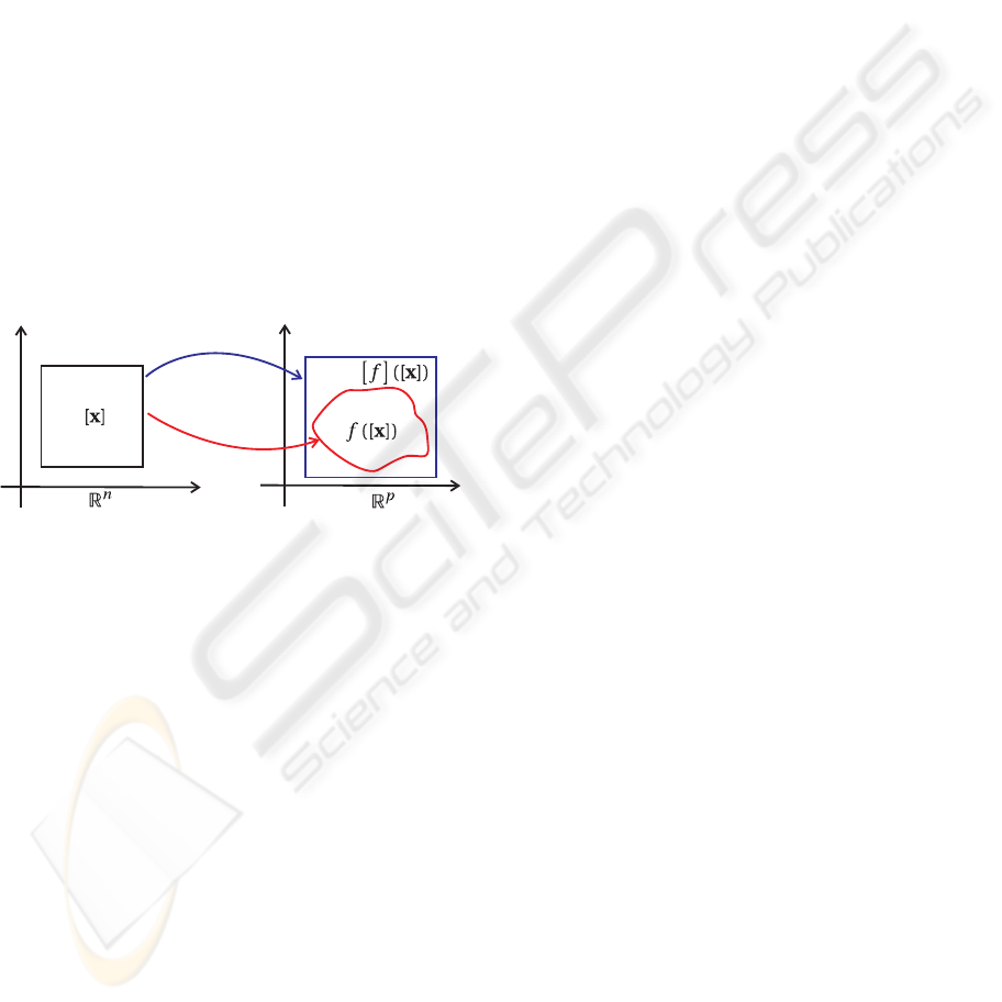
2.1 Inclusion Function
The function [f](.) : IR
n
→ IR
p
is an inclusion func-
tion of a function f :R
n
→ R
p
if
∀[x] ∈IR
n
, f([x]) , {f(x) | x ∈ [x]} ⊂ [f]([x]).
Illustration of inclusion function.
Interval computation makes it possible to obtain in-
clusion functions of a large class of nonlinear func-
tions, as illustrated by the following example.
Example 2 If f(x
1
, x
2
) ,
((1− 0.01x
2
)x
1
;(−1+ 0.02x
1
)x
2
), a methodology to
obtain an enclosure of the image set f([10, 20], [40, 50])
is as follows:
f
[40, 50]
[10, 20]
⊂
(1− 0.01∗ [40, 50]) ∗ [10, 20]
(−1+ 0.02∗ [10, 20]) ∗ [40, 50]
=
(1− [0.4, 0.5]) ∗ [10, 20]
(−1+ [0.2, 0.4]) ∗ [40, 50]
=
[0.5, 0.6] ∗ [10, 20]
[−0.8, −0.6] ∗ [40, 50]
=
([5, 12])
([−40, −24])
.
This methodology can easily be applied for any box
[x
1
] × [x
2
] and the resulting algorithm corresponds to
an inclusion function for f.
The interval union [x] ⊔ [y] of two boxes [x] and [y]
is the smallest box which contains the union [x] ∪ [y].
The width w([x]) of a box [x] is the length of its largest
side.
The ε-inflation of a box [x] = [x
−
1
, x
+
1
] × ·· · × [x
−
n
, x
+
n
] is
defined by
inflate([x], ε) , [x
−
1
− ε, x
+
1
+ ε] × · ··
··· × [x
−
n
− ε, x
+
n
+ ε]. (4)
2.2 Picard Theorem
Interval analysis for ordinary differential equations
were introduced by Moore (Moore, 1966) (See (Ne-
dialkov et al., 1999) for a description and a bibliog-
raphy on this topic). These methods provide numeri-
cally reliable enclosures of the exact solution of dif-
fential equations. These techniques are based on Pi-
card Theorem.
Theorem 1 Let t
1
be a positive real number. Assume
that x(0) is known to belong to the box [x](0). Assume
that u(t) ∈ [u] for all t ∈ [0, t
1
]. Let [w] be a box (that
is expected to enclose the path x(τ), τ ∈ [0, t
1
]). If
[x](0) + [0, t
1
] ∗ [f]([w], [u]) ⊂ [w], (5)
where [f]([x].[u]) is an inclusion function of f(x, u),
then, for all t ∈ [0, t
1
]
x([0, t
1
]) ⊂ [x](0) + [0, t
1
] ∗ [f]([w], [u]). (6)
2.3 Interval Flow
Definition: The inclusion function of the flow is a
function
[φ] :
IR × IR
n
× IR
m
→ IR
n
([t], [x], [u]) → [φ]([t], [x], [u])
such that
∀t ∈ [t], ∀x ∈ [x], u ∈F ([t] → [u]),φ(t, x, u) ∈ [φ]([t], [x], [u])
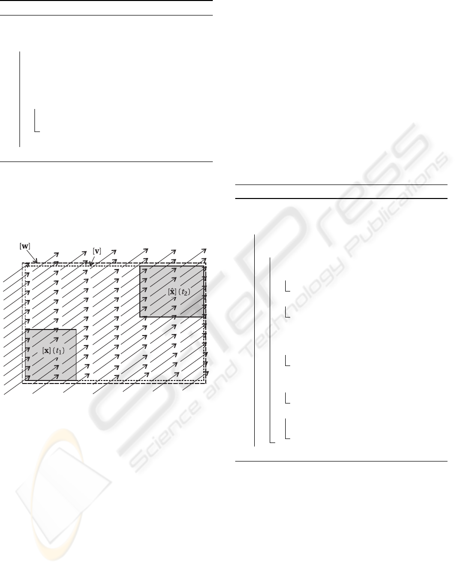
Using Theorem 1, one can build an algorithm com-
puting an enclosure [x]([t]) for the path x([t]) =
{
x(t), t ∈ [t]
}
from an enclosure [x] for x(0). The
principle of this algorithm is illustrated by Figure 1.
Comments : The interval [t] = [t
1
, t
2
] is such that
t
1
≥ 0. Step 2 computes an estimation [
ˆ
x](t
2
) for
the domain of all x(t
1
) consistent with the fact that
x(0) ∈ [x]. Note that, at this level, it is not certain that
[
ˆ
x](t
2
) contains x(t
2
). Step 3 computes the smallest
box [v] containing [x](t
1
) and [
ˆ
x](t
2
). At Step 4, [v] is
inflated (see (4)) to provide a good candidate for [w].
α and β are small positive numbers. Step 5 checks the
condition of Theorem 1. If the condition is not satis-
fied, no bounds can be computed for x(t
2
) and R
n
is
returned. Otherwise, Step 8 computes a box contain-
ing x(t
2
) using theorem 1.
ICINCO 2007 - International Conference on Informatics in Control, Automation and Robotics
6
Algorithm 1: Inclusion function [φ.]
Data: [t] = [t
1
, t
2
], [x](t
1
), [u]
Result: [x](t
2
)
begin1
[
ˆ
x](t
2
) := [x](t
1
) + (t
2
−t
1
) ∗ [f]([x](t
1
), [u]);2
[v] := [x](t
1
) ⊔ [
ˆ
x](t
2
);3
[w] := inflate([v],α.w([v]) + β);4
if [x](t
1
) + [0, t
2
−t
1
] ∗ [f]([w], [u]) * [w]5
then
[x](t
2
) := R
n
6
return7
[x](t
2
) := [x](t
1
) + (t
2
−t
1
) ∗ [f]([w], [u]);8
end9
The algorithm to we gave to compute the interval
flow is very conservative. The pessimism can drasti-
cally be reduced by using the Lohner method (Lohner,
1987).
Figure 1: Principle of algorithm [φ].
3 ALGORITHM
This section presents an algorithm to compute an in-
ner and an outer approximation of the capture basin.
It is based on Theorem 2.
Theorem 2 If C
−
and C
+
are such that C
−
⊂
C ⊂ C
+
⊂ K, if [x] is a box and if u ∈ F ([0, t] → U),
then
(i) [x] ⊂ T ⇒ [x] ⊂ C
(ii) [x] ∩ K =
/
0 ⇒ [x] ∩ C =
/
0
(iii)
φ(t, [x], u) ⊂ C
−
∧ φ([0, t], [x], u) ⊂ K
⇒ [x] ⊂ C
(iv) φ(t, [x], U)∩C
+
=
/
0∧φ(t, [x], U)∩K =
/
0 ⇒ [x]∩C =
/
0
Proof : (i) and (ii) are due to the inclusion
T ⊂ C ⊂ K. Since T ⊂ C
−
⊂ C, (iii) is a consequence
of the definition of the capture basin (see (3)). The
proof of (iv) is easily obtained by considering (3) and
in view of fact that C ⊂ C
+
⊂ K.
Finally, a simple but efficient bisection algorithm is
then easily constructed. It is summarized in Algo-
rithm 2. The algorithm computes both an inner and
outer approximation of the capture basin C. In what
follows, we shall assume that the set U of feasible in-
put vectors is a box [u]. The box [x] to be given as an
input argument for ENCLOSE should contain set K.
Comments. Steps 4 and 7 uses Theorem 2, (i)-(iii)
to inflate C
−
. Steps 5 and 8 uses Theorem 2, (ii)-(iv)
to deflate C
+
.
Algorithm 2: ENCLOSE.
Data: K, T, [x]
Result: C
−
, C
+
begin
C
−
←
/
0;C
+
← [x];L ←
{
[x]
}
;1
while
L 6=
/
0 do2
pop the largest box [x] from L ;3
if [x] ⊂ T then4
C
−
← C
−
∪ [x];
else if [x] ∩ K =
/
0 then5
C
+
← C
+
\[x];
take t ≥ 0 and u ∈ U6
if [φ](t, [x], u) ⊂ C
−
and7
[φ]([0, t], [x], u) ⊂ K then
C
−
← C
−
∪ [x];
else if [φ](t, [x], u) ∩ C
+
=
/
0 and8
[φ](t, [x], U) ∩ K =
/
0 then
C
+
← C
+
\[x];
else if w([x]) ≥ ε then9
bisect [x] and store the two resulting
boxes into
L ;
end
where
ε : ENCLOSE stops the bisecting procedure
when the precision is reached ;
C
−
: Subpaving (list of nonoverlapping boxes) rep-
resenting an inner approximation of the cap-
ture basin, that is the boxes inside the capture
basin C ;
C
+
: Subpaving representing the outer approx-
imation of the capture basin, that is the
boxes outside C and the boxes for which no
conclusion could be reached;
INNER AND OUTER APPROXIMATION OF CAPTURE BASIN USING INTERVAL ANALYSIS
7
These subpavings provide the following bracketing of
the solution set :
C
−
⊂ C ⊂ C
+
.
Figure 2: Two dimensional exemple of ENCLOSE algo-
rithm.
4 EXPERIMENTATIONS
This section presents an application of Algorithm 2.
The algorithm has been implemented in C + + using
Profil/BIAS interval library and executed on a Pen-
tiumM 1.4Ghz processor. As an illustration of the
algorithm we consider the Zermelo problem (Bryson
and Ho, 1975; Cardaliaguet et al., 1997). In control
theory, Zermelo has described the problem of a boat
which wants to reach an island from the bank of a
river with strong currents. The magnitude and direc-
tion of the currents are known as a function of posi-
tion. Let f(x
1
, x
2
) be the water current of the river at
position (x
1
, x
2
). The method for computing the ex-
pression of the speed vector field of two dimensional
flows can be found in (Batchelor, 2000). In our exam-
ple the dynamic is nonlinear,
f(x
1
, x
2
) ,
1+
x
2
2
− x
2
1
(x
2
1
+ x
2
2
)
2
,
−2x
1
x
2
(x
2
1
+ x
2
2
)
2
.
The speed vector field associated to the dynamic of
the currents is represented on Figure 3.
Let T ,
B (0, r) with r = 1 be the island and we set
K = [−8, 8] × [−4, 4], where K represents the river.
The boat has his own dynamic. He can sail in any
direction at a speed v. Figure 4 presents the two-
dimensional boat. Then, the global dynamic is given
by
x
′
1
(t) = 1+
x
2
2
− x
2
1
(x
2
1
+ x
2
2
)
2
+ vcos(θ)
x
′
2
(t) =
−2x
1
x
2
(x
2
1
+ x
2
2
)
2
+ vsin(θ)
,
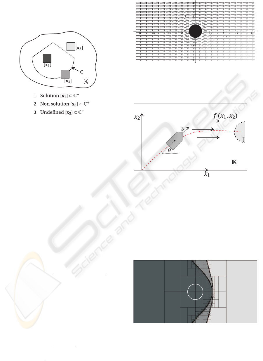
Figure 3: Vector field of the currents.
where the controls 0 ≤ v ≤ 0.8 and θ ∈ [−π, π].
Figure 4: Zermelo’s problem.
Figure 5 shows the result of the ENCLOSE algorithm,
where the circle delimits the border of the target T.
Then, C
−
corresponds to the union of all dark grey
boxes and C
+
corresponds to the union of both grey
and light grey boxes. Thus, we have the following
inclusion relation :
C
−
⊂ C ⊂ C
+
.
Figure 5: Two dimensional exemple of ENCLOSE algo-
rithm.
ICINCO 2007 - International Conference on Informatics in Control, Automation and Robotics
8

5 CONCLUSION
In this paper, a new approach to deal with capture
basin problems is presented. This approach uses inter-
val analysis to compute an inner an outer approxima-
tion of the capture basin for a given target. To fill out
this work, different perspectives appear. It could be
interesting to tackle problems in significantly larger
dimensions. The limitation is mainly due to the bi-
sections involved in the interval algorithms that makes
the complexity exponential with respect to the num-
ber of variables. Constraint propagation techniques
(L. Jaulin, M. Kieffer, O. Didrit, E. Walter, 2001)
make it possible to push back this frontier and to
deal with high dimensional problems (with more than
1000 variables for instance). In the future, we plan to
combine our algorithm with graph theory and guar-
anteed numerical integration (Nedialkov et al., 1999;
Delanoue, 2006) to compute a guaranteed control u.
ACKNOWLEDGEMENTS
The authors wish to thank N. Delanoue for many help-
ful comments and valuable discussions
REFERENCES
Aubin, J. (1991). Viability theory. Birkh
¨
auser, Boston.
Batchelor, G.-K. (2000). An introduction to fluid dynamics.
Cambridge university press.
Bryson, A. E. and Ho, Y.-C. (1975). Applied optimal control
: optimization, estimation, and control. Halsted Press.
Cardaliaguet, P., Quincampoix, M., and Saint-Pierre, P.
(1997). Optimal times for constrained nonlinear con-
trol problems without local controllability. Applied
Mathematics and Optimization, 36:21–42.
Cruck, E., Moitie, R., and Seube, N. (2001). Estima-
tion of basins of attraction for uncertain systems with
affine and lipschitz dynamics. Dynamics and Control,
11(3):211–227.
Delanoue, N. (2006). Algorithmes numriques pour
l’analyse topologique. PhD dissertation, Universit
´
e
d’Angers, ISTIA, France. Available at
www.istia.
univ-angers.fr/
˜
delanoue/
.
Kearfott, R. B. and Kreinovich, V., editors (1996). Appli-
cations of Interval Computations. Kluwer, Dordrecht,
the Netherlands.
L. Jaulin, M. Kieffer, O. Didrit, E. Walter (2001). Ap-
plied Interval Analysis, with Examples in Parameter
and State Estimation, Robust Control and Robotics.
Springer-Verlag, London.
Lohner, R. (1987). Enclosing the solutions of ordinary ini-
tial and boundary value problems. In Kaucher, E.,
Kulisch, U., and Ullrich, C., editors, Computer Arith-
metic: Scientific Computation and Programming Lan-
guages, pages 255–286. BG Teubner, Stuttgart, Ger-
many.
Moore, R. E. (1966). Interval Analysis. Prentice-Hall, En-
glewood Cliffs, NJ.
Nedialkov, N.-S., Jackson, K.-R., and Corliss, G.-F. (1999).
Validated solutions of initial value problems for ordi-
nary differential equations. Applied Mathematics and
Computation, 105:21–68.
Saint-Pierre, P. (1994). Approximation of the viability ker-
nel. Applied Mathematics & Optimization, 29:187–
209.
INNER AND OUTER APPROXIMATION OF CAPTURE BASIN USING INTERVAL ANALYSIS
9
