IMPLEMENTATION OF RECURRENT MULTI-MODELS FOR

SYSTEM IDENTIFICATION

Lamine Thiaw, Kurosh Madani

Laboratoire Image, Signal et Systmes Intelligents (LISSI / EA 3956) IUT de Snart, Universit Paris XII

Av. Pierre Point, F-77127 Lieusaint, France

Rachid Malti

Laboratoire Automatique Productique et Signal University Bordeaux 1 351, Cours de la Libration, 33405 Talence Cedex, France

Gustave Sow

LER, Ecole Suprieure Polytechnique de Dakar, Universit Cheikh Anta Diop, BP 5085, Dakar Fan, Senegal

Keywords:

System identiﬁcation, non-linear systems, multi-model, recurrent models.

Abstract:

Multi-modeling is a recent tool proposed for modeling complex nonlinear systems by the use of a combination

of relatively simple set of local models. Due to their simplicity, linear local models are mainly used in such

structures. In this work, multi-models having polynomial local models are described and applied in system

identiﬁcation. Estimation of model’s parameters is carried out using least squares algorithms which reduce

considerably computation time as compared to iterative algorithms. The proposed methodology is applied

to recurrent models implementation. NARMAX and NOE multi-models are implemented and compared to

their corresponding neural network implementations. Obtained results show that the proposed recurrent multi-

model architectures have many advantages over neural network models.

1 INTRODUCTION

Identiﬁcation of nonlinear systems is an important

task for many real world applications such as process

behavior analysis, control, prediction, etc. In the last

years, several classes of models have been developed,

among which Artiﬁcial Neural Networks (ANN) and

multi-models (also known as operating regime ap-

proach), for non linear system identiﬁcation.

ANN are widely used for dynamical nonlinear

system modeling (Cheng et al., 1997; Konur and

Okatan, 2004; Vartak et al., 2005). Such implementa-

tions like Time Delay Neural Network (TDNN) (Cor-

radini and Cohen, 2002; Konur and Okatan, 2004),

Jordan Network (Jordan, 1986), Elman Network (El-

man, 1999) are very suitable for time series appli-

cations but they suffer of some limitations which re-

strict their use (Huang et al., 2005; Tomasz and Jacek,

1997). Several papers have been dedicated to the en-

hancement of neural networks for recurrent models

identiﬁcation (Bielikova, 2005; Huang et al., 2006).

In (Huang et al., 2006) for example, a Multi-Context

Recurrent Neural Network (MCRN) is studied and its

performances are compared with those of the Elman

Network and Elman Tower Network. Even though

the proposed MCRN allows to achieve good perfor-

mances, the main drawback remains its complexity

due to the number of parameters induced by the con-

text layer (Huang et al., 2006) which has weighting

connections with both hidden and output layers.

The main difﬁculty encountered in recurrent neu-

ral networks is parameters estimation complexity.

The parameters estimation is mostly performed us-

ing the gradient descent method (Backpropagation

Through Time algorithm, Real Time Recurrent Learn-

ing algorithms, etc.) which cannot guarantee conver-

gence to global minimum. On the other hand, the re-

lated algorithm’s performance is very sensitive to the

learning rate parameter which determines the conver-

gence rate and the stability of the algorithm.

Multi-models have recently been proposed in nu-

merous papers (Boukhris et al., 2000; Vernieuwe

et al., 2004; Li et al., 2004) for modeling and con-

trol of nonlinear systems. For such systems, it is gen-

314

Thiaw L., Madani K., Malti R. and Sow G. (2007).

IMPLEMENTATION OF RECURRENT MULTI-MODELS FOR SYSTEM IDENTIFICATION.

In Proceedings of the Fourth International Conference on Informatics in Control, Automation and Robotics, pages 314-321

DOI: 10.5220/0001615503140321

 SciTePress

erally difﬁcult to ﬁnd a single analytical relationship

describing system’s behavior in its whole operating

range. The system’s complexity can be considerably

reduced if system’s operating range is divided into

different regions where local behavior could be de-

scribed with relatively simple models. The system’s

behavior is approximated by the weighted contribu-

tion of a set of local models. The difﬁculty encoun-

tered in this approach is the splitting of the system’s

operating range into convenient regions. For that pur-

pose, various techniques have been studied among

which grid partitioning, decision tree partitioning,

fuzzy clustering based partitioning (see (Vernieuwe

et al., 2004; Murray-Smith and Johansen, 1997)).

Fuzzy clustering based partitioning enables to gather

those data that may have some “similarities”, facilitat-

ing system’s local behavior handling. The main dif-

ﬁculty is the number of clusters needed to determine

the multi-model’s architecture. A method is presented

here to bypass this difﬁculty.

Parameter estimation of recurrent multi-models is

much simpler as compared to recurrent neural net-

works. We present in this work a multi-model imple-

mentation of recurrent models with polynomial local

models. The proposed structure is applied to NAR-

MAX and NOE models. The main advantage of such

structure is that it allows to adjust the complexity of

local models to the detriment of global one and vice-

versa. Parameters are estimated using least squares

algorithms, avoiding time consuming calculations and

local minima.

The paper is structured as follows: in section 2

an overview of models identiﬁcation principle is pre-

sented. Section 3 describes the general principle of

multi-models using polynomial local models. The im-

plementation of recurrent multi-model is presented in

section 4. Results and discussions are presented in

section 5.

2 OVERVIEW OF NON LINEAR

MODELS

“Black box” models are very suited for complex sys-

tems representation (Sjoberg et al., 1995). Identiﬁca-

tion of such models consists of determining the math-

ematical relationship linking system’s outputs (or its

states) to its inputs from experimental data. In gen-

eral, model describing system’s behavior

can be ex-

Multi-input and single-output (MISO) systems are con-

sidered here for ease of understanding. Results can be gen-

eralized to multi-input and multi-output systems.

pressed as:

y(t + h) = F



u(t), ˜y(t)



+ e(t + h) (1)

where :

y(t + h) is the unknown system output at time instant

t + h;

t is the current time instant and h is the prediction

step;

(·) is an unknown deterministic nonlinear function

describing the system (the true model);

u(t) is a column vector which components are sys-

tem’s inputs at time t and at previous time instants;

˜y(t) is a column vector which components are ob-

tained from system’s output at time t and at previous

time instants. It can be built from measured output

data, estimated output data, prediction errors, or

simulation errors;

e(t + h) is an error term at time t + h.

The identiﬁcation task consists of determining the

function F(·) which is the best approximation of F

(·)

and estimating the system’s output ˆy:

ˆy(t + h) = F



u(t), ˜y(t),θ



= F



ϕ(t),θ



(2)

where :

ϕ(t) = [u(t)

, ˜y(t)

]

is the regression vector ob-

tained by the concatenation of the elements of vectors

u(t) and ˜y(t); and θ is a parameter vector to be esti-

mated.

If ˜y(t) in (2) depends on model’s output or model’s

states, then the model (2) is said to be recurrent. Re-

current models have the ability to take into account

system’s dynamics. On the other hand, data col-

lected from a process are usually noisy due to the

sensors or the inﬂuence of external factors. Recur-

rent models allow to obtain unbiased parameters esti-

mation. Various model classes have been established

for modeling dynamical systems in presence of vari-

ous noise conﬁgurations. Model classes differ by the

composition of their regression vector. Since the ex-

act model class is frequently unknown various classes

are usually tested and the best one is chosen. In this

work we focus on recurrent models called Nonlinear

AutoRegressive Moving Average with eXogenous in-

puts (NARMAX) and Nonlinear Output Error (NOE)

models. These classes of models are widely used be-

cause of their ability to capture nonlinear behaviors.

NARMAX model is a very powerful tool for mod-

eling and prediction of dynamical systems (Gao and

Foss, 2005; Johansen and Er, 1993; Yang et al., 2005).

It is well suited for modeling systems using noisy out-

puts and noisy states. It generalizes the Nonlinear Au-

toRegressive with eXogenous inputs (NARX) model.

Its regression vector is composed of the past inputs

IMPLEMENTATION OF RECURRENT MULTI-MODELS FOR SYSTEM IDENTIFICATION

315

, the past measured outputs y

, and the past pre-

diction errors (difference between measured and pre-

dicted outputs) e. The output of the NARMAX model

is given by:

y(t + 1) = F



(t − d

+ 1),.. .,

...

(t − d

+ 1),.. .,u

(t − d

− n

+ 2)

...

(t − d

+ 1).. .,y

(t − d

− n

+ 2),

e(t − d

+ 1),.. .,e(t − d

− n

+ 2)



+e(t + 1) (3)

where:

, d

and d

are inputs, output, and error delays re-

spectively;

, n

and n

are inputs, output, and error orders re-

spectively;

The prediction step in this representation corresponds

to:

h = min(d

) (4)

A NOE model is suited for system’s simulation

because it does not require measured outputs (Palma

and Magni, 2004). The corresponding regression vec-

tor is composed of past inputs u

and past simulated

outputs ˆy

. The output of the NOE model is given by:

y(t + 1) = F



(t − d

+ 1),.. .,

...

(t − d

+ 1),.. .,u

(t − d

− n

+ 2)

...

ˆy

(t − d

ˆy

+ 1),.. ., ˆy

(t − d

ˆy

− n

ˆy

+ 2)



+e(t + 1) (5)

Identiﬁcation of recurrent models such as NAR-

MAX or NOE models is a difﬁcult task because some

of the regressors have to be computed at each time

step. The parameter estimation must then be carried

out recursively.

3 MULTI-MODEL’S PRINCIPLE

Multi-models were ﬁrst proposed by Johansen and

Foss in 1992 (Johansen and Er, 1992). A multi-model

is a system representation composed by a set of local

models each of which is valid in a well deﬁned fea-

ture space corresponding to a part of global system’s

behavior. The local validity of a model is speciﬁed by

an activation function which tends to 1 in the feature

space and tends to zero outside. The whole system’s

behavior can then be described by the combination of

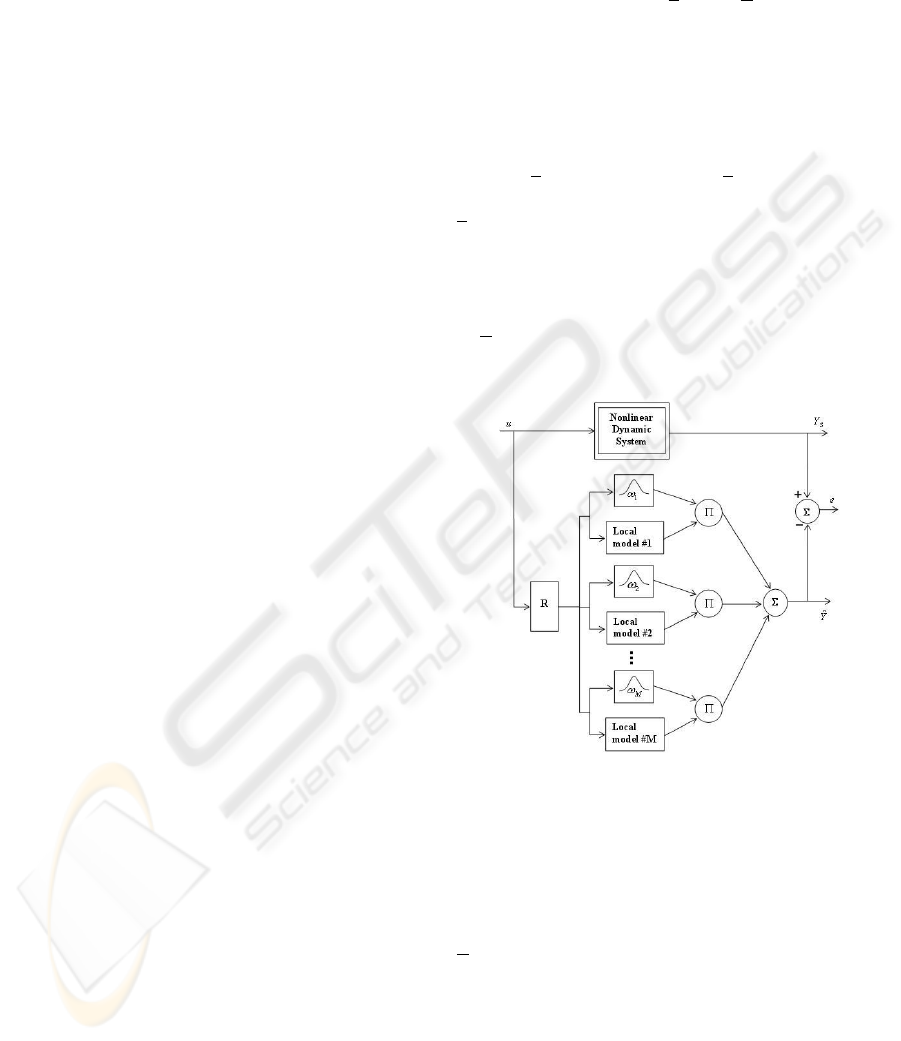
all local models outputs. Figure 1 presents the basic

architecture of a multi-model. The relation (2) can

then be expressed as:

ˆy(t + h) =

∑

i=1



(t)





ϕ(t),θ



(6)

where:

M is the number of local models;

(·) is the activation degree of local model f

(·),

with :



ξ(t)



∈ [0, 1] ,

∑

i=1



ξ(t)



= 1 ∀t

ξ(t) is the vector of indexing variables (variables

whereby system’s feature space is divided into sub-

spaces (Orjuela et al., 2006));

is a parameter vector characterizing the local model

(·);



ϕ(t),θ



= ˆy

(t + h) is the predicted output of the

ith local model.

In (6), the prediction step h may take any discrete

Figure 1: Basic architecture of a multi-model. Bloc R is a

set of time delay operators combined with a linear or nonlin-

ear transformation and used for the regression vector con-

struction; Y

is the measured system output.

value. It can also be speciﬁed by an appropriate

choice of the time delays d

, d

and d

of regressors in

ϕ(t) (see equation (4)). So without loss of generality,

we will assume that h = 1.

Activation degrees of local models can be de-

ﬁned in a deterministic way using membership func-

tions like gaussian functions, sigmoidal functions,

etc. They can also be deﬁned fuzzily using a fuzzy

clustering of the system’s feature space. This lat-

ter solution seems to be more natural as it allows to

gather data which may have some “similarities”. The

main difﬁculty is the determination of the number of

ICINCO 2007 - International Conference on Informatics in Control, Automation and Robotics

316

clusters. The proposed implementation combines ar-

chitectural (number of local models or clusters) and

parametrical identiﬁcation. The number of clusters is

successively incremented and the parameters are esti-

mated at each step. The incrementation of the number

of clusters is stopped when Akaike Information Cri-

terion (see section §5) starts deteriorating.

The “fuzzy-c-means” algorithm (Bezdec, 1973)

is implemented here because of its simplicity. This

algorithm consists of maximizing the intra-cluster

similarities and minimizing the inter-cluster similari-

ties. The corresponding objective function is deﬁned

as:

J(c

,. ..,c

) =

∑

i=1

∑

t=1

(7)

where:

= kϕ(t)− c

k denotes the distance between the ob-

servation ϕ(t) (t = 1,. .., N, N - number of observa-

tions) and the center c

of the ith cluster (i = 1,.. ., M,

M - number of clusters or local models);

∑

k=1

(

)

2/(m−1)

represents membership degree of

the observation ϕ(t) in the cluster i and stands for the

local model’s activation degree for that observation:

= ω



ξ(t)



;

∑

t=1

∑

t=1

ϕ(t)

is the center of the ith cluster;

m ≥ 1 is the “fuzzy exponent” and represents the over-

lapping shape between clusters (generally, m = 2).

Local models may be of any structural type. As

suggested in (Johansen and Er, 1993), local mod-

els may be deﬁned as the ﬁrst p terms of the Tay-

lor’s series expansion of the true (unknown) model

(·) about a point located in the local model’s feature

space. Afﬁne local models (p = 1) are mostly used

because of their simplicity. This multi-model struc-

ture is very close to Takagi-Sugeno one. For com-

plex systems, the number of linear local models may

be very important because of the simplicity of their

structure. We propose in this work polynomial local

models with p ≥ 1 which enable to enhance the han-

dling of local nonlinearities, reducing then the num-

ber of models. We use a nonlinear transformation of

the regression vector:

(t) = g



ϕ(t)



where g

(·) is a nonlinear transformation producing

the new regression vector ϕ

(t) which components

are the products of elements of ϕ(t) at orders 1 to p.

(t) can be easily obtained from the following pro-

cedure:

Let

ϕ(t) = [ϕ

·· · ϕ

]

(8)

where n

is the dimension of ϕ(t).

Let us consider the following row vectors:

1,1

= [ϕ

··· ϕ

]

1,2

= [ϕ

··· ϕ

]

...

1,n

= [ϕ

]

2,1

= [ϕ

1,1

1,2

··· ϕ

1,n

]

2,2

= [ϕ

1,2

··· ϕ

1,n

]

...

2,n

= [ϕ

1,n

]

...

p−1,1

= [ϕ

p−2,1

p−2,2

··· ϕ

p−2,n

]

p−1,2

= [ϕ

p−2,2

··· ϕ

p−2,n

]

...

p−1,n

= [ϕ

p−2,n

]

p,1

= [ϕ

p−1,1

p−1,2

··· ϕ

p−1,n

]

(t) is then obtained from the relation:

(t) = [V

1,1

2,1

·· · V

p,1

]

(9)

For example if ϕ(t) = [ϕ

]

and p = 2, then

relation (9) gives:

(t) = [ϕ

]

The number of parameters n

of ϕ

(t) may be very

important if the size of ϕ(t) is important or if the order

p is high.

For notation simplicity we will replace V

k,1

by V

Local models can then be expressed by the relation:



ϕ(t),θ



∑

k=1

+ θ

(10)

where:

(k = 0 ·· ·n

and i = 1 ···M) are real constants;

= [θ

·· · θ

]

parameters vector of the

ith local model.

The main advantage of such a representation is that

local models are nonlinear whereas they are linear

with respect to parameters. This structure consider-

ably simpliﬁes parameter estimation (see §4). Equa-

tion (6) can be rewritten as:

ˆy(t + 1) = Φ(t)

θ (11)

where:

Φ(t) =



ξ(t)



(t)

·· ·ω



ξ(t)



(t)

is the

global weighted regression vector;

(t) =



(t)



is the extended regression vector;

θ =



.. .θ



is a concatenation of all local

models parameters vectors;

IMPLEMENTATION OF RECURRENT MULTI-MODELS FOR SYSTEM IDENTIFICATION

317

Estimating θ can be carried out by using a global

learning criteria J which consists of minimizing the

error between system’s output and multi-model’s out-

put:

J =

∑

t=1



(t) − ˆy(t)



∑

t=1



ε(t)



(12)

For non-recurrent multi-models with polynomial

local models, J is linear with respect to the multi-

model’s parameters vector. J is minimized analyti-

cally using Least-Squares method. Multi-model pa-

rameters are then computed using the expression:

θ = (Φ

)

−1

(Φ

) (13)

where:

θ is the estimation of θ;



Φ(t)



t=N

t=1

is global weighted regression matrix

of all observations;



(t)



t=N

t=1

is the vector of output values of all

observations;

For recurrent multi-models, parameters are esti-

mated by a parametrical adaptation algorithm using

at each time step the values of Φ(t), y

(t) and ω

[ξ(t)]

as presented in the next section.

4 MULTI-MODEL’S

IMPLEMENTATION OF

RECURRENT MODELS

Parameter estimation in recurrent neural network

models is carried out iteratively using gradient based

algorithm. Convergence towards global minimum is

not guaranteed and convergence rate might be high.

As it will be stated here, for the proposed recurrent

multi-model (RMM), parameters are estimated using

recursive least squares. Hence, the criterion J in re-

lation (12) is computed up to time step k according

to:

J(k) =

∑

t=1



ε(t)



∑

t=1



(t) − Φ

(t − 1) θ



(14)

with θ

the value of θ evaluated up to time instant k.

The minimization of this criterion leads to:

∑

t=1

Φ(t − 1) Φ

(t − 1)

−1

∑

t=1

(t)Φ(t − 1)

(15)

Relation (15) can be written in a recursive form.

Assuming

∑

t=1

Φ(t − 1) Φ

(t − 1)

−1

(16)

then

= A

∑

t=1

(t)Φ(t − 1) (17)

k+1

= A

k+1

∑

t=1

(t)Φ(t − 1) (18)

The sum in the right hand side of (18) can be trans-

formed after some manipulations to:

k+1

∑

t=1

(t)Φ(t − 1) = A

−1

k+1

+ Φ(k)

ε(k + 1) (19)

where:

ε(k + 1) = y

(k + 1)− Φ

(k) θ

is the a priori predic-

tion error (the error at time instant k+1 evaluated with

parameters computed up to time instant k). Putting

(19) in (18) leeds to a recursive expression of θ:

k+1

= θ

+ A

k+1

Φ(k)

ε(k + 1) (20)

k+1

can also be computed recursively. From (16)

one can write :

k+1

]

−1

= [A

]

−1

+ Φ(k)Φ

(k) (21)

Applying matrix inversion lemma to relation (21),

k+1

is computed recursively:

k+1

= A

−

Φ(k) Φ

(k) A

1 + Φ

(k) A

Φ(k)

(22)

So, the parameters vector θ is updated recursively

at each time step using relations (22) and (20). This

learning algorithm is used for the identiﬁcation of

NARMAX and NOE structures based on the RMM

architectures (see ﬁgures 2 and 3).

Figure 2: Recurrent multi-model implementation of a NAR-

MAX model.

ICINCO 2007 - International Conference on Informatics in Control, Automation and Robotics

318

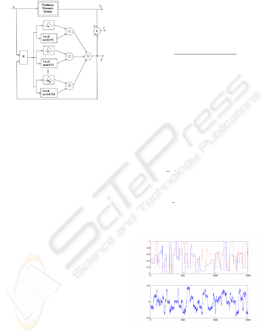
Figure 3: Recurrent multi-model implementation of a NOE

model.

5 RESULTS AND DISCUSSION

To validate the proposed RMM architecture, two non

linear systems are used. The ﬁrst one is a simulated

system which data are generated from a NARX model

(Gasso, 2000). The second one is Box-Jenkins gas

furnace benchmark (Box and Jenkins, 1970). For

comparison purposes, we have implemented recur-

rent Multi-Layer Perceptron (MLP) with one hidden

layer for NARMAX and NOE models, both trained

with the Backpropagation Through Time (BPTT) al-

gorithm (Werbos, 1990). To enhance the speed of

learning with the BBTT algorithm, the learning rate

is adapted so that it takes high values when the learn-

ing error decreases fastly and take small values when

it decreases slowly.

Performances of recurrent multi-models with

given order p of polynomial local models (RMM

)

are evaluated. Akaike Information Criterion (AIC)

is used for model’s parsimony estimation (least error

with minimum parameters):

AIC = N lnJ + 2 n

(23)

where n

denotes the number of model’s parameters.

Root Mean Square Error criterion (RMSE) is also

used for performance evaluation in learning (RMSE

)

and validation (RMSE

) phases. The architecture of

models (Arch) speciﬁes the number of local models in

multi-models case or the number of hidden neurons

in MLP case. Computation time (CT) during which

models parameters are determined is used for algo-

rithms convergence speed evaluation.

5.1 Example 1: Narx Dynamic Process

The following system is simulated in a noisy context

and then identiﬁed using recurrent multi-model and

recurrent MLP.

(t) =

(t−1)



0.5u

(t−1)−0.3u

(t−1)



1+y

(t−1)

+0.3u

(t − 1) − 0.5u

(t − 1) (24)

Exogenous input signals u

(·) and u

(·) are cho-

sen to be pulses of random magnitude (in interval

[0,1]) and different widths; the output signal is then

corrupted by a white noise e issued from a normal dis-

tribution. The signal to noise ratio equals 14 dB. The

obtained noisy output y

(see ﬁgure 4) is expressed

by:

(t) = y

(t) + e(t) (25)

NOE model class is the most suitable one to iden-

tify this kind of system (Dreyfus, 2002). Both NOE

RMM and NOE MLP models are implemented. The

following regression vector is used:

ϕ(t) = [u(t − 1) ˆy(t − 1)]

where ˆy is the estimated model output. The vector of

indexing variables is:

ξ(t) =



(t) u

(t)



Table 1 shows obtained results for NOE RMMs and a

NOE MLP structures. System and NOE RMM

out-

puts are plot on validation data in ﬁgure 5. The ob-

Figure 4: Inputs and output indentiﬁcation data.

tained results show that multi-model structures have

performances equivalent to MLP structures. How-

ever, their computation time is much lower.

IMPLEMENTATION OF RECURRENT MULTI-MODELS FOR SYSTEM IDENTIFICATION

319

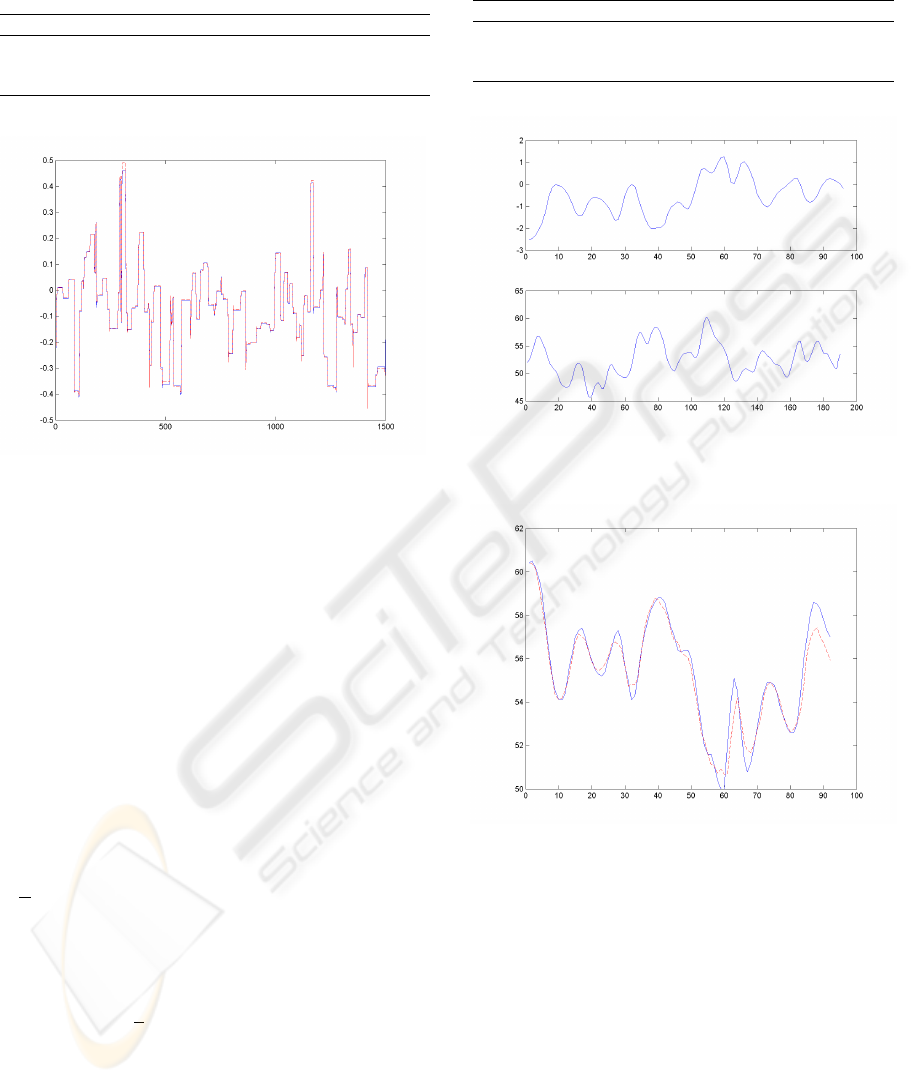
Table 1: NOE model for the nonlinear dynamic process:

results for NOE RMM and NOE MLP structures.

Model Arch. AIC CT(s) RMSE

RMSE

RMM

7 -9595 8 0.040 0.010

RMM

3 -9617 6 0.040 0.007

MLP 3 -9587 199 0.040 0.006

Figure 5: NOE RMM

output (dotted line) and noise free

system output on validation data.

5.2 Example 2: Box-Jenkins Gas

Furnace Benchmark

In this benchmark, data set are obtained from a com-

bustion process of methane-air mixture. The pro-

cess input is the methane gas ﬂow into the furnace

and the output is CO

concentration in the outlet gas

(Box and Jenkins, 1970). System inputs and outputs

are presented in ﬁgure 6. We have implemented and

compared a NARMAX MLP and a NARMAX RMM

structures based on the described methodologies. The

following regression vector is used:

ϕ(t) = [u(t − 1) u(t − 2) u(t − 3)

(t − 1) y

(t − 2) y

(t − 3) e(t − 1)]

The vector of indexing variables is:

ξ(t) =



u(t) y

(t)



The results are presented in table 2. The NARMAX

RMM has the best parsimony and gives best perfor-

mances on validation data, with a very low computa-

tion time compared to the NARMAX MLP. It can be

seen that high polynomial orders reduces the number

of local models. Figure 7 shows process and NAR-

MAX RMM

outputs on validation data.

Table 2: NARMAX model for Box-Jenkins gas furnace

data: results for Multi-model and MLP structures.

Model Arch. AIC CT(s) RMSE

RMSE

RMM

6 -692 3 0.12 0.55

RMM

2 -637 2 0.13 0.63

MLP 3 -622 35 0.17 0.58

Figure 6: Process input and output on identiﬁcation data.

Figure 7: Process and NARMAX RMM

(dotted line) out-

puts on validation data.

6 CONCLUSION

In this work, a new recurrent multi-model structure

with polynomial local models is proposed. The ad-

vantage of using polynomial local models is a better

handling of local nonlinearities and reducing hence-

forth the number of local models. The proposed struc-

ture is used to implement NARMAX and NOE mod-

els.

Identiﬁcation task is carried out very simply and

obtained results show that the proposed recurrent

multi-model has many advantages over recurrent

ICINCO 2007 - International Conference on Informatics in Control, Automation and Robotics

320

MLP model, among which the reduction of compu-

tation time. This is due to the way the parameters are

estimated: least squares formula in the former model

and iterative algorithm in the latter.

The perspective of this study is the implementa-

tion of the proposed structures for model predictive

control in industrial processes.

REFERENCES

Bezdec, J. (1973). Fuzzy mathematics in pattern classiﬁca-

tion. PhD thesis, Applied Math. Center, Cornell Uni-

versity Ithaca.

Bielikova, M. (2005). Recurrent neural network training

with the extended kalman ﬁlter. IIT. SRC, pages 57–

64.

Boukhris, A., Mourot, G., and Ragot, J. (2000). Nonlin-

ear dynamic system identiﬁcation: a multiple-model

approach. Int. J. of control, 72(7/8):591–604.

Box, G. and Jenkins, G. (1970). Time series analysis,

forecasting and control. San Francisco, Holden Day,

pages 532–533.

Cheng, Y., Karjala, T., and Himmelblau, D. (1997). Closed

loop nonlinear process identiﬁcation using internal re-

current nets. Neural Networks, 10(3):573–586.

Corradini, A. and Cohen, P. (2002). Multimodal speech-

gesture interface for hands-free painting on virtual pa-

per using partial recurrent neural networks for gesture

recognition. in Proc. of the Int’l Joint Conf. on Neural

Networks (IJCNN’02), 3:2293–2298.

Dreyfus, G. (2002). Rseaux de Neurones - Mthodologie et

applications. Eyrolles.

Elman, J. (1999). Finding structure in time. Cognitive Sci-

ence, 14(2):179–211.

Gao, Y. and Foss, A. (2005). Narmax time series model

prediction: feed forward and recurrent fuzzy neural

network approaches. Fuzzy Sets and Sytems, 150:331–

350.

Gasso, K. (2000). Identiﬁcation de systmes dynamiques non

linaires: approche multi - modle. thse de doctorat de

l’INPL.

Huang, B., Rashid, T., and Kechadi, M.-T. (2005). A recur-

rent neural network recognizer for online recognition

of handwritten symbols. ICEIS, 2:27–34.

Huang, B., Rashid, T., and Kechadi, M.-T. (2006). Multi-

context recurrent neural network for time series appli-

cations. International Journal of Computational In-

telligence, 3(1):45–54.

Johansen, T. and Er, M. (1992). Nonlinear local model rep-

resentation for adaptive systems. In Proc. of the IEEE

Conf. on Intelligent Control and Instrumentation, vol-

ume 2, pages 677–682, Singapore.

Johansen, T. and Er, M. (1993). Constructing narmax using

armax. Int. Journal of Control, 58(5):1125–1153.

Jordan, M. (1986). Attractor dynamics and parallelism in

a connectionist sequential machine. In Proceedings

of IASTED International Conference of the Cognitive

Science Society. (Reprinted in IEEE Tutorials Series,

New York: IEEE Publishing Services, 1990), pages

531–546, Englewood Cliffs, NJ: Erlbaum.

Konur, U. and Okatan, A. (2004). Time series prediction

using recurrent neural network architectures and time

delay neural networks. ENFORMATIKA, pages 1305–

1313.

Li, N., Li, S. Y., and Xi, Y. G. (2004). Multi-model predic-

tive control based on the takagi-sugeno fuzzy models:

a case study. Information Sciences, 165:247–263.

Murray-Smith, R. and Johansen, T. (1997). Multiple Model

Approaches to Modeling and Control. Taylor and

Francis Publishers.

Orjuela, R., Maquin, D., and Ragot, J. (2006). Identiﬁca-

tion des systmes non linaires par une approche multi-

modle tats dcoupls. Journes Identiﬁcation et Modli-

sation Exprimentale JIME’2006 - 16 et 17 novembre -

Poitiers.

Palma, F. D. and Magni, L. (2004). A multimodel struc-

ture for model predictive control. Annual Reviews in

Control, 28:47–52.

Sjoberg, J., Zhang, Q., Ljung, L., Benveniste, A., De-

lyon, B., Glorennec, P., Hjalmarsson, H., and Judit-

sky, A. (1995). Nonlinear black-box modeling in sys-

tem identiﬁcation: a uniﬁed overview. Automatica 31,

31(12):1691–1724.

Tomasz, J. and Jacek, M. (1997). Neural networks tool for

stellar light prediction. In Proc. of the IEEE Aerospace

Conference, volume 3, pages 415–422, Snowmass,

Colorado, USA.

Vartak, A., Georgiopoulos, M., and Anagnostopoulos, G.

(2005). On-line gauss-newton-based learning for

fully recurrent neural networks. Nonlinear Analysis,

63:867–876.

Vernieuwe, H., Georgieva, O., Baets, B., Pauwels, V., Ver-

hoest, N., and Troch, F. (2004). Comparison of data-

driven takagi-sugeno models of rainfall-discharge dy-

namics. Journal of Hydrology, XX:1–14.

Werbos, P. (1990). Backpropagation through time: What

it does and how to do it. Proceedings of the IEEE,

78(10):1550–1560.

Yang, W. Z., L.H., Y., and L., C. (2005). Narmax model

representation and its application to damage detection

for multi-layer composites. Composite Structures,

68:109–117.

IMPLEMENTATION OF RECURRENT MULTI-MODELS FOR SYSTEM IDENTIFICATION

321