
DOMAIN-SPECIFIC MODELLING WITH ATOM
3
Hans Vangheluwe, Ximeng Sun and Eric Bodden
School of Computer Science, McGill University, Montr
´
eal, Qu
´
ebec, Canada
Keywords:
Meta-modelling, model transformation, domain-specific modelling, traffic simulation.
Abstract:
Using domain-specific modelling environments maximally constrains users, matching their mental model of
the problem domain, and allows them to only build syntactically correct models. Anecdotal evidence shows
that domain-specific modelling can drastically improve productivity as well as product quality. In this paper,
the foundations of (domain-specific) modelling language design are presented. Our guiding principle is to
“model everything”. It is indeed shown how all aspects of language design can be explicitly (meta-)modelled
enabling the efficient synthesis of domain-specific, visual, modelling environments. The case of AToM
3
, A
Tool for Multi-formalism and Meta Modelling, is elaborated. Concepts are illustrated by modelling, analysis,
simulation, and eventual synthesis of software for Traffic networks.
1 DISSECTING A MODELLING
LANGUAGE
To explicitly model domain-specific modelling lan-
guages and ultimately synthesize visual modelling en-
vironments for those, we will break down a modelling
language into its basic constituents. The following is
based on a description by Harel and Rumpe (Harel
and Rumpe, 2000), taking common programming lan-
guage concepts and putting them in a more general
modelling context. An earlier version of this section
appeared as a tutorial at a 2006 MoDELS workshop
(Giese et al., 2006).
The two main aspects of a model are its syntax
(how it is represented) on the one hand and its seman-
tics (what it means) on the other hand.
The syntax of modelling languages is traditionally
partitioned into concrete syntax and abstract syntax.
In textual languages for example, the concrete syn-
tax is made up of sequences of characters taken from
an alphabet. These characters are typically grouped
into words or tokens. Certain sequences of words or
sentences are considered valid (i.e., belong to the lan-
guage). The (possibly infinite) set of all valid sen-
tences is said to make up the language. Costagliola
et. al. (Costagliola et al., 2002) present a framework
of visual language classes in which the analogy be-
tween textual and visual characters, words, and sen-
tences becomes apparent. Visual languages are those
languages whose concrete syntax is visual (graphi-
cal, geometrical, topological, ...) as opposed to tex-
tual. For practical reasons, models are often stripped
of irrelevant concrete syntax information during syn-
tax checking. This results in an “abstract” representa-
tion which captures the “essence” of the model. This
is called the abstract syntax. Obviously, a single ab-
stract syntax may be represented using multiple con-
crete syntaxes. In programming language compil-
ers, abstract syntax of models (due to the nature of
programs) is typically represented in Abstract Syntax
Trees (ASTs). As in the context of general modelling,
models are often graph-like, this representation can be
generalized to Abstract Syntax Graphs (ASGs). Once
the syntactic correctness of a model has been estab-
lished, its meaning must be specified. This meaning
must be unique and precise (to allow correct model
exchange and code synthesis for example). Meaning
can be expressed by specifying a semantic mapping
function which maps every model in a language onto
an element in a semantic domain. For example, the
meaning of Activity Diagrams may be given by map-
ping it onto Petri Nets. For practical reasons, seman-
305
Vangheluwe H., Sun X. and Bodden E. (2007).
DOMAIN-SPECIFIC MODELLING WITH ATOM.
In Proceedings of the Second International Conference on Software and Data Technologies, pages 305-314
DOI: 10.5220/0001346903050314
Copyright
c
SciTePress

tic mapping is usually applied to the abstract rather
than to the concrete syntax of a model. Note that the
semantic domain is a modelling language in its own
right which needs to be properly modelled (and so on,
recursively). In practice (in tools), the semantic map-
ping function maps abstract syntax onto abstract syn-
tax.
To continue this introduction of meta-modelling
and model transformation concepts, languages will
explictly be represented as (possibly infinite) as
shown in Figure 1. In the figure, insideness denotes
the sub-set relationship. The dots represent models
which are elements of the encompassing set(s). As
one can always, at some level of abstraction, represent
a model as a graph structure, all models are shown as
elements of the set of all graphs
Graph. Though this
restriction is not necessary, it is commonly used as
it allows for the elegant design, implementation and
bootstrapping of (meta-)modelling environments. As
such, any modelling language becomes a (possibly
infinite) set of graphs. In the bottom centre of Fig-
ure 1 is the abstract syntax set
A. It is a set of models
stripped of their concrete syntax.
Meta-modelling is a heavily over-used term. Here,
we will use it to denote the explicit description (in
the form of a finite model in an appropriate meta-
modelling language) of the abstract syntax set
A of
a modelling language. Often, meta-modelling also
covers a model of the concrete syntax. Semantics
is however not covered. In the figure, the set
A is
described by means of the model
meta-model of A.
On the one hand, a meta-model can be used to check
whether a general model (a graph) belongs to the set
A. On the other hand, one could, at least in principle,
use a meta-model to generate all elements of
A. This
explains why the term meta-model and grammar are
often used inter-changeably.
Several languages are suitable to describe meta-
models. Two approaches are in common use:
1. A meta-model is a type-graph. Elements of the
language described by the meta-model are in-
stance graphs. There must be a morphism be-
tween an instance-graph (model) and a type-graph
(meta-model) for the model to be in the language.
Commonly used meta-modelling languages are
Entity Relationship Diagrams (ERDs) and Class
Diagrams (adding inheritance to ERDs). The ex-
pressive power of this approach is often not suffi-
cient and an extra constraint language (such as the
Object Constraint Language (OCL) in the UML)
specifying constraints over instances is used to
further specify the set of models in a language
(adding the expressive power of first or higher or-
der logic). This is the approach used by the OMG
to specify the abstract syntax of the UML.
2. An alternative general approach specifies a meta-
model as a transformation (in an appropriate for-
malism such as Graph Grammars (Rozenberg,
1997)) which, when applied to a model, veri-
fies its membership of a formalism by reduc-
tion. This is similar to the syntax checking based
on (context-free) grammars used in programming
language compiler compilers. Note how this ap-
proach can be used to model type inferencing and
other more sophisticated checks.
Both types of meta-models (type-graph or gram-
mar) can be interpreted (for flexibility and dynamic
modification) or compiled (for performance). Note
that when meta-modelling is used to synthesize in-
teractive, possibly visual modelling environments, we
need to model when to check whether a model be-
longs to a language. In free-hand modelling, checking
is only done when explicitly requested. This means
that it is possible to create, during modelling, syn-
tactically incorrect models. In syntax-directed mod-
elling, syntactic constraints are enforced at all times
during editing to prevent a user from creating syn-
tactically incorrect models. Note how the latter ap-
proach, though possibly more efficient, due to its in-
cremental nature –of construction and consequently
of checking– may render certain valid models in the
modelling language unreachable through incremen-
tal construction. Typically, syntax-directed modelling
environments will be able to give suggestions to mod-
ellers whenever choices with a finite number of op-
tions present themselves.
The advantages of meta-modelling are numerous.
First, an explicit model of a modelling language can
serve as documentation and as specification. Such
a specification can be the basis for the analysis of
properties of models in the language. From the
meta-model, a modelling environment may be auto-
matically generated. The flexibility of the approach
is tremendous: new, possibly domain-specific, lan-
guages can be designed by simply modifying parts of a
meta-model. As this modification is explicitly applied
to models, the relationship between different vari-
ants of a modelling language is apparent. Above all,
with an appropriate meta-modelling tool, modifying
a meta-model and subsequently generating a possibly
visual modelling tool is orders of magnitude faster
than developing such a tool by hand. The tool syn-
thesis is repeatable and less error-prone than hand-
crafting. As a meta-model is a model in an appropri-
ate modelling language in its own right, one should
be able to meta-model that language’s abstract syn-
tax too. Such a model of a meta-modelling language
is called a meta-meta-model. This is depicted in Fig-
ICSOFT 2007 - International Conference on Software and Data Technologies
306
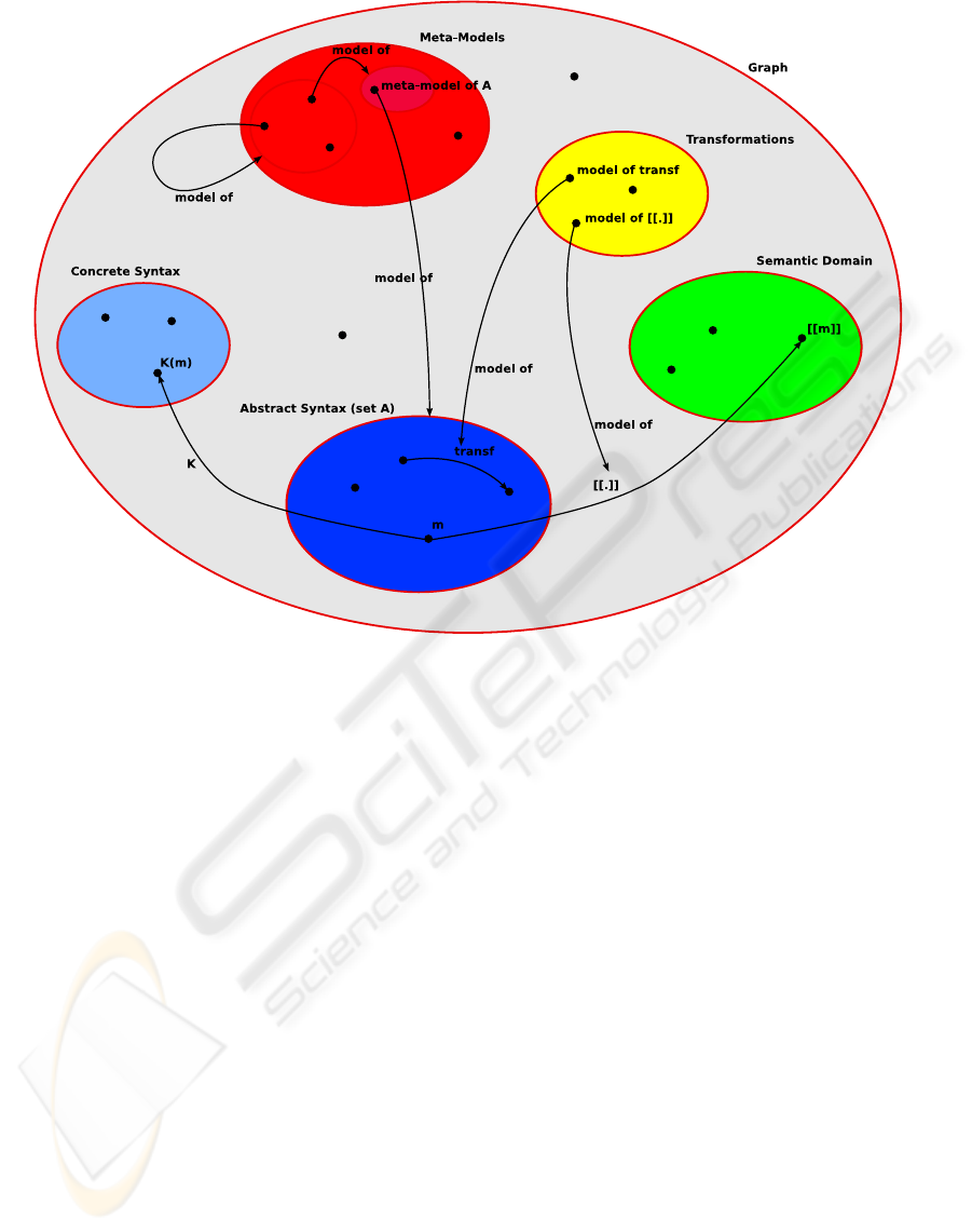
Figure 1: Modelling Languages as Sets.
ure 1. It is noted that the notion of “meta-” is relative.
In principle, one could continue the meta- hierarchy
ad infinitum. Luckily, some modelling languages can
be meta-modelled by means of a model in the lan-
guage itself. This meta-circularity allows modelling
tool and language compiler builders to bootstrap their
systems.
A model
m in the Abstract Syntax set (see Fig-
ure 1) needs at least one concrete syntax. This implies
that a concrete syntax mapping function κ is needed.
κ maps an abstract syntax graph onto a concrete syn-
tax model. Such a model could be textual (e.g., an
element of the set of all Strings), or visual (e.g., an el-
ement of the set of all the 2D vector drawings). Note
that the set of concrete models can be modelled in its
own right. It is noted that grammars may be used to
model a visual concrete syntax (Minas, 2002). Also,
concrete syntax sets will typically be re-used for dif-
ferent languages. Often, multiple concrete syntaxes
will be defined for a single abstract syntax, depend-
ing on the intended user. If exchange between mod-
elling tools is intended, an XML-based textual syntax
is appropriate. If in such an exchange, space and per-
formance is an issue, a binary format may be used in-
stead. When the formalism is graph-like as in the case
of a circuit diagram, a visual concrete syntax is often
used for human consumption. The concrete syntax of
complex languages is however rarely entirely visual.
When for example equations need to be represented,
a textual concrete syntax is more appropriate.
Finally, a model
m in the Abstract Syntax set (see
Figure 1) needs a unique and precise meaning. This is
achieved by providing a Semantic Domain and a se-
mantic mapping function
[[.]]
. This mapping can
be given informally in English, pragmatically with
code or formally with model transformations. Natu-
ral languages are ambiguous and not very useful since
they cannot be executed. Code is executable, but it
is often hard to understand, analyze and maintain. It
can be very hard to understand, manage and derive
properties from code. This is why formalisms such as
Graph Grammars are often used to specify semantic
mapping functions in particular and model transfor-
mations in general. Graph Grammars are a visual for-
malism for specifying transformations. Graph Gram-
mars are formally defined and at a higher level than
code. Complex behavior can be expressed very intu-
itively with a few graphical rules. Furthermore, Graph
Grammar models can be analyzed and executed. As
efficient execution may be an issue, Graph Grammars
DOMAIN-SPECIFIC MODELLING WITH ATOM3
307

can often be seen as an executable specification for
manual coding. As such, they can be used to auto-
matically generate transformation unit tests.
Not only semantic mapping, but also general model
transformations can be explicitly modelled as illus-
trated by
—transf— and its model in Figure 1. It is
noted that models can be transformed between differ-
ent formalisms.
Within the context of this paper, we have chosen
to use the following terminology (see also (Giese et
al., 2006)).
• A language is the set of abstract syntax models.
No meaning is given to these models.
• A concrete language comprises both the abstract
syntax and a concrete syntax mapping function
κ. Obviously, a single language may have several
concrete languages associated with it.
• A formalism consists of a language, a semantic
domain and a semantic mapping function giving
meaning to model in the language.
• A concrete formalism comprises a formalism to-
gether with a concrete syntax mapping function.
We will also focus on our tool AToM
3
(Lara and
Vangheluwe, 2002). It is noted that several other
meta-environment toolsets exists (see for example
www.meta-environment.org
). We use our tool as
it closely follows the general framework described
above.
Many challenges still remain for Model Driven
Engineering. As with programs, models evolve over
time. Model version control, based on computing
model differences is necessary. As even meta-models
and models transformations (in particular, of seman-
tics) may evolve, this must also be dealt with.
2 MODELLING TRAFFIC
NETWORKS
Domain- and formalism-specific modelling have the
potential to greatly improve productivity (Kelly and
Tolvanen, 2000). They are able to exploit features in-
herent to a specific domain or formalism. This will
for example enable specific analysis techniques or the
synthesis of efficient code. The time required to con-
struct such domain/formalism-specific modelling and
simulation environments can however be prohibitive.
Thus, rather than using such specific environments,
generic environments are typically used. Those are
necessarily a compromise.
To illustrate domain-specific modelling, we intro-
duce a simplified
TimedTraffic formalism, a visual no-
tation specific to the vehicle traffic domain (Papa-
costas and Prevedouros, 1992). It is of course possi-
ble to model traffic systems using a variety of generic
modelling and simulation languages such as
GPSS,
DEVS (Zeigler, 1984), and Petri Nets. We choose
not to do this, but rather build a
TimedTraffic-specific
modelling environment. This maximally constrains
users, allowing them, by construction, to only build
syntactically and, for as far as this can be statically
checked, semantically correct models. Furthermore,
the
TimedTraffic-specific, visual syntax used matches
the users’ mental model of the problem domain.
Figure 2 shows a lattice of traffic-related For-
malisms and relevant transformations between them.
At the top is
TimedTraffic, a domain-specific formal-
ism allowing the description of timed movement of
cars through a traffic network. A modeller may wish
to visualize the dynamics of a traffic systems, ana-
lyze properties such as liveness, and obtain perfor-
mance metrics such as average throughput. To sup-
port this variety of goals, Figure 2 shows how
Timed-
Traffic
is mapped onto different formalisms. When
timing information is removed from a model, a con-
servative abstraction, an untimed
Traffic model is ob-
tained. As shown in (Vangheluwe and Lara, 2004),
an appropriate transformation onto
Petri Nets then al-
lows for analysis of pertinent properties such as live-
ness and conservation. For timed analysis, mapping
onto
Timed Transition Petri Nets may be done. For
performance analysis by means of simulation, map-
ping onto the DEVS formalism (and simulation us-
ing for example the pythonDEVS tool) is appropri-
ate. Although desirable, implementing modelling en-
vironments which support the formalisms and trans-
formations in Figure 2 seems a daunting task. The
meta-modelling and model transformation concepts
described in the previous section can however be used
to model all formalisms and transformations. We
have implemented the entire figure but for brevity will
demonstrate the principles of our approach by show-
ing the meta-model and the operational semantics of
TimedTraffic.
2.1 Modelling TimedTraffic
A modelling environment for the domain-specific for-
malism
TimedTraffic allows users to model traffic flow
by means of connected road segments, cars and traf-
fic lights. Traffic signals impose constraints on how
cars can be moved by this transformation. Further-
more, the model is timed, i.e., cars move at a certain
constant speed (in our chosen abstraction) and traffic
lights switch state every fixed number of time units.
We first introduce the abstract syntax of
Timed-
Traffic
and explain how it can be modelled within the
ICSOFT 2007 - International Conference on Software and Data Technologies
308
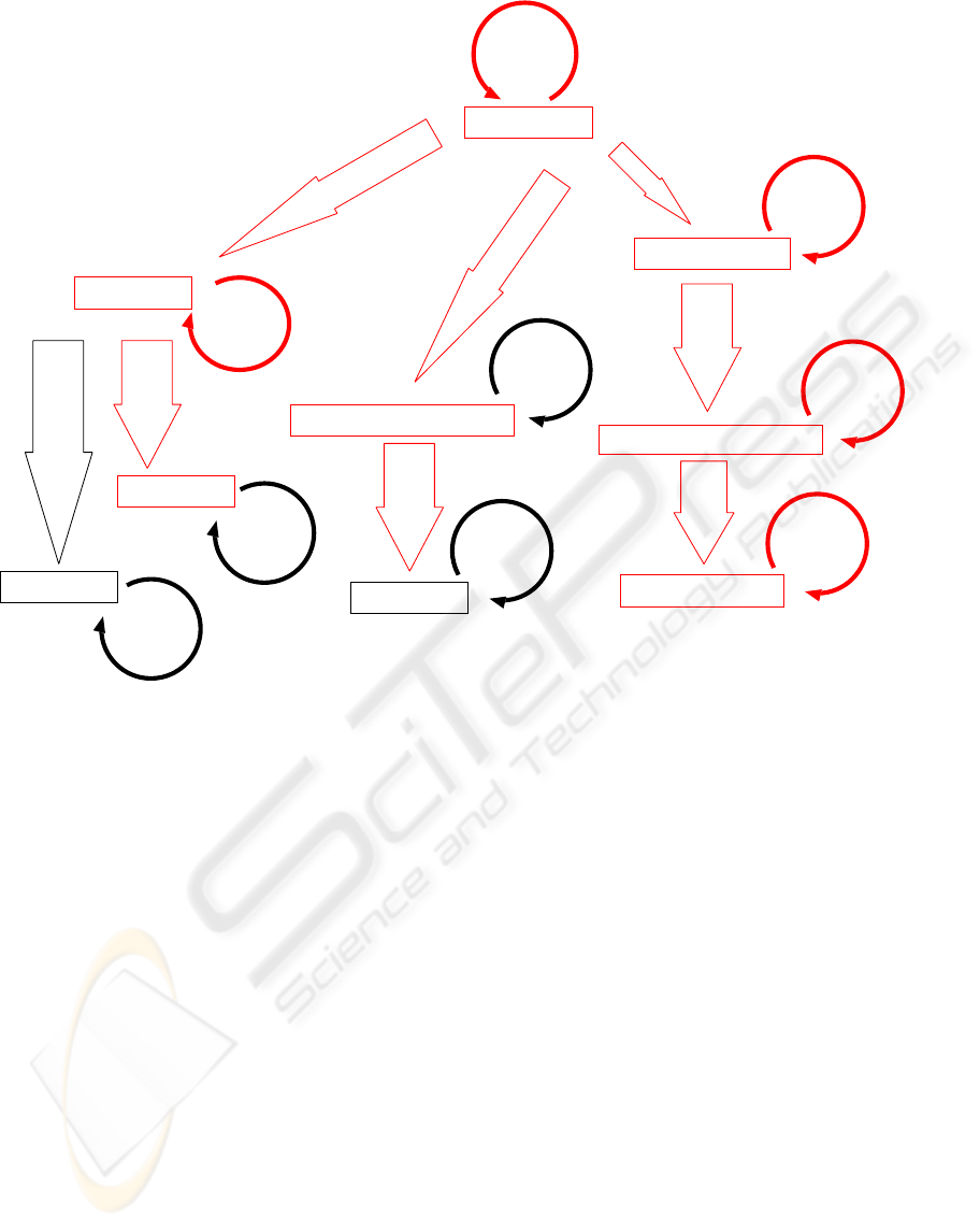
neglect time
Traffic (un-timed)
Place-Transition Petri Nets
Coverability Graph
describe semantics
by mapping onto
compute all
possible behaviours
simulate
simulate
analyze:
reachability,
coverability, ...
describe semantics
by mapping onto
simulate
DEVS
map onto
map onto
Timed Transition Petri Nets
describe semantics
by mapping onto
simulate
analyze
describe semantics
by mapping onto
TINA
simulate
analyze
pythonDEVS
simulate
DEVSJava
simulate
TimedTraffic
simulate
Figure 2: Various Traffic formalisms and transformations between them.
AToM
3
modelling environment, along with the static
semantics which imposes certain non-behavioural
constraints. We then show how concrete syntax in-
formation can be added to allow synthesis of a visual
modelling tool for
TimedTraffic. We also demonstrate
how concrete syntax can change over time to reflect
state changes on the abstract level. We finally model
(operational) semantics of this formalism by means
of a graph grammar which describes how cars move
through a given traffic network.
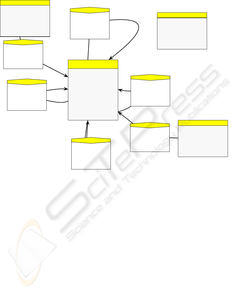
2.1.1 Abstract Syntax
The abstract syntax model or meta-model of
Timed-
Traffic
is shown as a model in the Entity Relationship
formalism in Figure 3. This ER meta-model com-
prises the following entities and relations:
roadSegment Can be connected to other road seg-
ments. Also, since our model is a timed model, road
segments have a size to determine the time a car needs
to cross them. A road segment may also have a finite
capacity.
car Each car can move almost independently through
the network. “Almost” because a car is not allowed
to cross a road segment which has a connected traf-
fic light showing red. A car has a certain fixed speed
and based on this and the length of a road segment,
a “schedule time” can be computed which gives the
time of its next move, relative to the last move time.
For informational purposes, we also include a global
event time, which shows the global timestamp of the
next scheduled move.
trafficLight A traffic light in our simple model can
have two states, red and green. Just like cars, they
have a schedule time, which reflects the time of their
next state change.
globalInfo This is singleton global entity for informa-
tional purposes showing the global time during the
simulation.
relations There are multiple types of associations
which indicate which entities may be connected.
These impose multiplicity constraints: a road segment
can only be connected to at most one other road seg-
ment per direction (top, bottom, left, right). This is
enforced by setting cardinalities
To roadSegment:
0 to 1
and
From roadSegment: 0 to 1
.
The abstract syntax induced by this metamodel
rigorously defines all entities, their attributes, their
DOMAIN-SPECIFIC MODELLING WITH ATOM3
309
Attributes:
- Length :: Integer
- capacity :: Integer
Constraints:
> initsetting
Cardinalities:
- From carLink: 0 to N
- From lightLink: 0 to N
- To roadTop: 0 to N
- From roadTop: 0 to N
- To roadLeft: 0 to N
- From roadLeft: 0 to N
- To roadRight: 0 to N
- From roadRight: 0 to N
- To roadBottom: 0 to N
- From roadBottom: 0 to N
roadSegment
Attributes:
- plateno :: String
- speed :: Integer
- scheduletime :: Integer
- globalEventTime :: Integer
Cardinalities:
- To carLink: 0 to N
car
Attributes:
- currentstate :: Enum
- scheduletime :: Integer
- direction :: Enum
Cardinalities:
- To lightLink: 0 to N
trafficlight
Attributes:
- globalTime :: Integer
globalInfo
roadLeft
Attributes:
- linkType :: String
Actions:
> connecting
> disconnecting
Cardinalities:
- To roadSegment: 0 to 1
- From roadSegment: 0 to 1
roadRight
Attributes:
- linkType :: String
Constraints:
> connecting
> disconnecting
Cardinalities:
- To roadSegment: 0 to 1
- From roadSegment: 0 to 1
lightLink
Attributes:
- linkType :: String
Cardinalities:
- To roadSegment: 0 to 1
- From trafficlight: 0 to 2
carLink
Attributes:
- linkType :: String
Cardinalities:
- To roadSegment: 0 to N
- From car: 0 to N
roadBottom
Attributes:
- linkType :: String
Constraints:
> connecting
> disconnecting
Cardinalities:
- To roadSegment: 0 to 1
- From roadSegment: 0 to 1
roadTop
Attributes:
- linkType :: String
Constraints:
> connecting
> disconnecting
Cardinalities:
- To roadSegment: 0 to 1
- From roadSegment: 0 to 1
Figure 3: Metamodel for the abstract syntax of Timed traffic.
possible connections and constraints amongst them.
The user of the modelling environment for
TimedTraf-
fic
is however probably more concerned with the con-
crete syntax. In the following, we show how such a
concrete syntax can be given to each abstract counter-
part using AToM
3
.
2.1.2 Concrete Syntax
Cars are rendered as a simple icon (constructed in
AToM
3
’s icon editor drawing tool) showing a bird’s
eye view of a car. On top the car’s global move time is
displayed. See Fig. 6 for an example. Road segments,
as mentioned above, can be connected to zero to one
other road segments on each side. To reflect which
each road segment is connected to, each such segment
contains four arrows, each of which is made visible
when the segment is being connected and made in-
visible on disconnection. The effect of this is seen
in Fig. 6, where only those arrows are visible that re-
late to existing connections. In addition to the con-
crete syntax (an icon) for each entity, a concrete syn-
tax needs to be associated with each association. Two
types of concrete syntax are typically used. On the
one hand, associations can be rendered by means of
geometric constraints. Connected road segments will
for example be visually placed next to one another.
On the other hand, a spline with a pointed arrow may
be used as in the case of the connection between a
traffic light and a road segment. A traffic light is mod-
elled by a traffic light icon along with two textual la-
bels showing the current state and the number of time
units until the next state switch. The actual switch
is triggered by a graph grammar action as described
below.
One concrete instance of a
TimedTraffic model is
shown in figure 6 which also shows how it evolves
over time. This behaviour is modelled in a graph
grammar which we explain in the following section.
2.1.3 Operational Semantics (Behaviour)
The transformation of models is a crucial element
in all model-based endeavours. As models, meta-
models, and meta-meta-models are all in essence at-
tributed, typed graphs, we can transform them by
ICSOFT 2007 - International Conference on Software and Data Technologies
310

means of graph rewriting. The rewriting is specified
in the form of
Graph Grammar models. These are
a generalization, for graphs, of Chomsky grammars.
They are composed of rules. Each rule consists of
Left Hand Side (LHS) and Right Hand Side (RHS)
graphs. Rules are evaluated against an input graph,
called the host graph. If a matching is found between
the LHS of a rule and a sub-graph of the host graph,
then the rule can be applied. When a rule is applied,
the matching subgraph of the host graph is replaced
by the RHS of the rule. Rules can have applicability
conditions, as well as actions to be performed when
the rule is applied. Some graph rewriting systems
have control mechanisms to determine the order in
which rules are checked. After a rule matching and
subsequent application, the graph rewriting system
starts the search again. The graph grammar execution
ends when no more matching rules are found.
The behaviour of any syntactically valid
Timed-
Traffic
model is given by a set of Graph Grammar
rules. Each car has an initial “next move time”. After
each move (caused by a graph grammar rule) we re-
calculate the next move time based on the car’s
speed
attribute and the
length
attribute of the road segment
that has been moved to. We can thus calculate the
next move time of each car:
car.nextMoveTime =
targetRoadSegment.length
car.speed
(1)
Note that this move time is relative: it gives the num-
ber of time units until its next move. Consequently, a
car can be moved whenever its next move time is zero
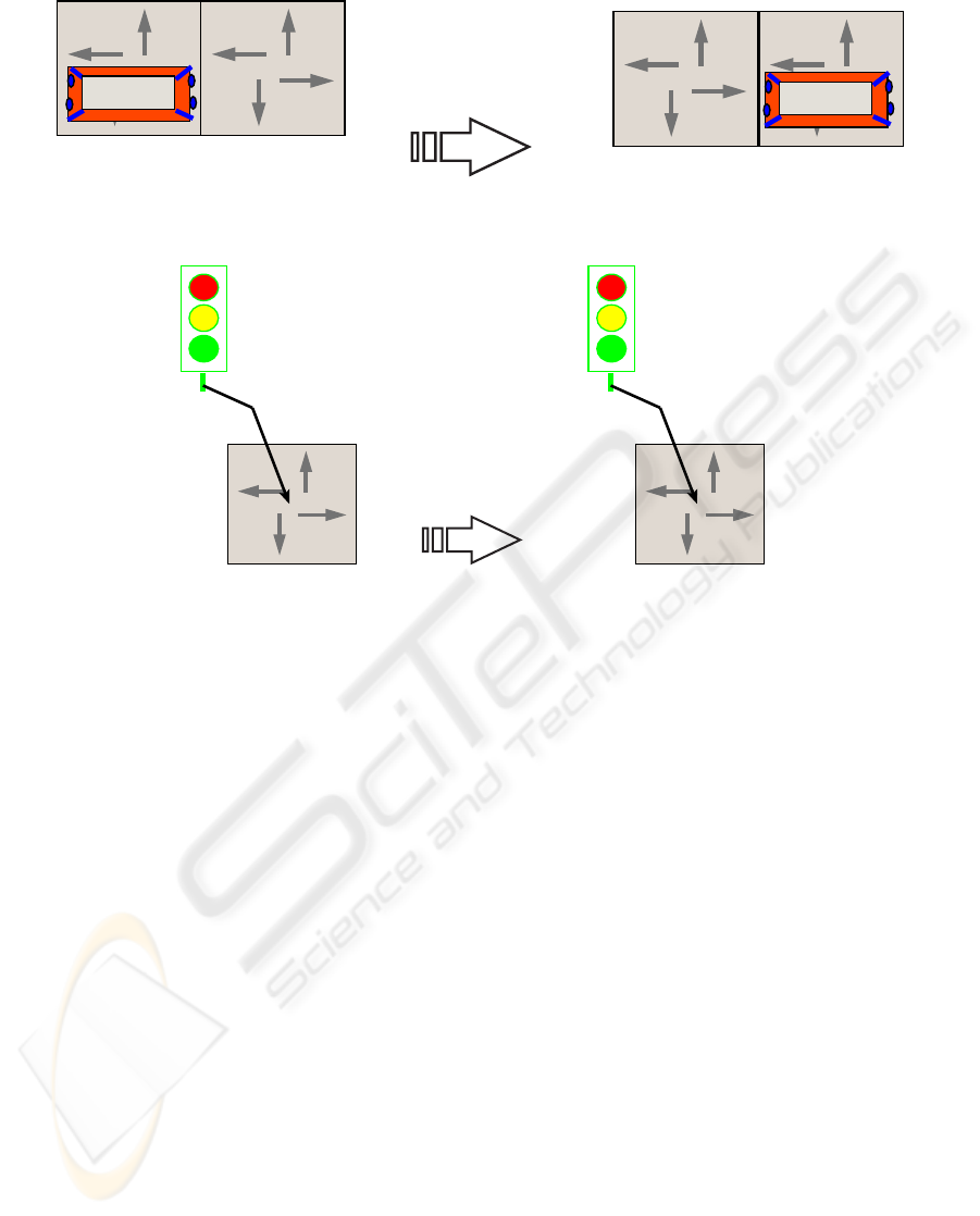
(unless it is blocked due to a red light). The rule in
Fig. 4 reflects this transformation when a car is moved
to the right.
The rule has a condition (not shown here) that the
schedule time must be 0 for this rule to apply. A fur-
ther condition states that all traffic lights (if any) con-
nected to the right road segment (where the car in-
tends to move) should be in state green and the capac-
ity of that road segment should not have been reached.
The rule itself consists of a LHS which identifies the
situation which should be matched. Each abstract en-
tity is assigned a label (a number): (1) left road seg-
ment; (2) right road segment; (3) car; (4) connection
between road segments (left to right); (5) connection
between road segments (right to left); (6) connection
between car and left road segment. The rule moves
the car by replacing matched entities. If a label on
the RHS occurs on the LHS this means that it reflects
the same entity. If it is a new label, it means that a
new entity was created. If a label appears on the LHS
and not on the RHS, an entity was deleted. In this ex-
ample, 6 was removed and a connection 8 was added,
this time connecting the car to the right road segment.
The (concrete syntax) constraint solver running in the
background takes care of actually moving the car vi-
sually once the connection changes. Also, after the
move, the new schedule time is calculated according
to equation 1. The AToM
3
modelling tool reflects this
by showing
<SPECIFIED>
on the RHS of each rule,
i.e., the new move time attribute is specified by the
rule. There are similar rules for moving cars left, up,
and down.
We also need to define the timed behaviour of the
traffic lights. We do so as shown in Fig. 5. Each time
the
lefttime
reaches 0, the rule applies and switches
the traffic light’s state. In our very simple model, we
then set the new “lefttime” to 10. The figure shows the
rule for switching to green. There is also a similar rule
for switching to red. The calculation of time progress
is contained in a seventh rule which only contains ac-
tions given in the pseudo-code below:
minScheduleTime = MAX
for each car in cars:
if car.scheduleTime < minScheduleTime:
minScheduleTime = minScheduleTime
for each light in trafficLights:
if light.scheduleTime < minScheduleTime:
minScheduleTime = minScheduleTime
globalTime += minScheduleTime
for each car in cars:
car.scheduleTime -= minScheduleTime
for each light in trafficLights:
light.scheduleTime -= minScheduleTime
First the minimal schedule time over all cars and
traffic lights is calculated. Then the global time is ad-
vanced by this offset and the offset is subtracted from
the schedule times of all the cars and traffic lights
(saturating at 0 to allow blocked cars), i.e., we make
time progress. Note that this leaves at least one car or
traffic light with a schedule time of 0, which means
that one of the other transformation rules can apply
to actually move the car or switch the light respec-
tively. The seven transformation rules are ordered in
the graph grammar with the following priorities:
1. turn light (red/green)
2. move car (left/right/up/down)
3. reschedule
This leads to the fact that first all traffic lights with a
schedule time of 0 are switched. If there is no such
light or all have been switched already, then all cars
with a schedule time of 0 are moved. Since all “move”
rules have the same priority, the move direction is ran-
dom (within the constraints given by connected red
traffic lights). Finally, when all such cars are moved
we know that no light or car with schedule time 0 ex-
ists any more and hence we can safely advance time
by applying (i.e., matching) the last rule.
DOMAIN-SPECIFIC MODELLING WITH ATOM3
311
<ANY>
1 2
3
4
6
5
<SPECIFIED>
1 2
3
4
8
5
Figure 4: MoveRight rule.
red
0
State:
Lefttime:
3
2
1
green
10
State:
Lefttime:
3
2
1
Figure 5: Light behaviour.
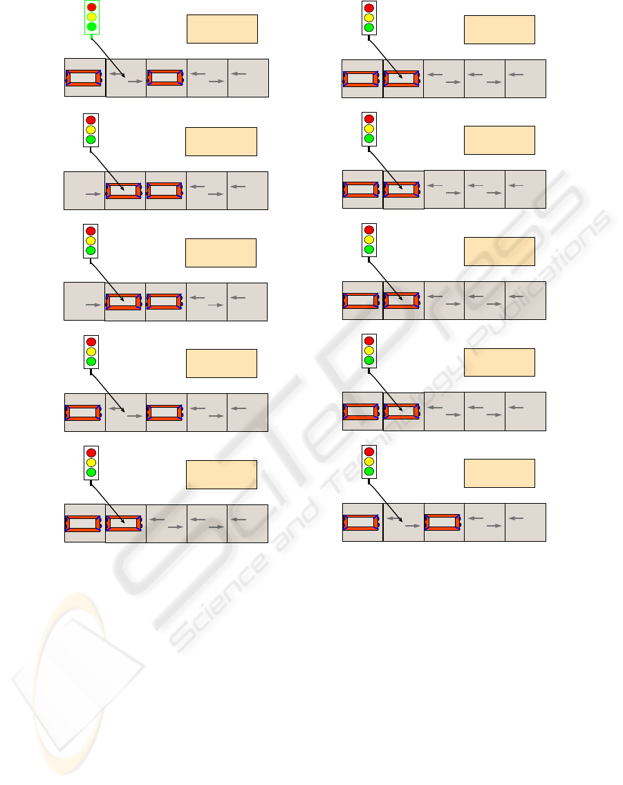
2.1.4 Example Simulation
An example of applying some steps of the transfor-
mation is shown in Figure 6 (to be read top to bottom,
left to right). We start with the traffic light showing
green and a schedule time of 10 time units. The left
car (with a speed of 10) is about to move and the right
car (with a speed of 3) is to be moved in 4 time units.
The size of each road segment is 40. According to the
priorities stated above, the first match we obtain is the
rule moving the left car to the right, since its schedule
time is 0. Afterwards, only the last rule can be applied
and hence we reschedule, which leads to the third sub-
figure. Note that the new schedule time for the moved
car is again 4 by equation (1). In this state, both cars
can move since for both the move time is 4, which
equals the global time (i.e., for both, the offset is 0
and one of the “move” rules can apply). Here, non-
deterministically, the left car is chosen and is moved
back again, leading to the fourth sub-figure. The next
move time for this car is now 8, by equation (1). In
the next step, the second car is moved to the left and
also its next move time is recalculated. According to
the same equation, this time we calculate a time of
17, adding 40/3 = 13 to the previous move time 4.
Then, no more cars can move and so time is incre-
mented by applying the “reschedule” rule. After do-
ing so, the schedule time of the traffic light becomes 0
which means that in the subsequent step, the state of
this light can be switched to “red”. Then again time
passes until the global time 17 (one but last subfigure)
which enables the second car to move. This simula-
tion could be executed over an arbitrary amount of
time and indeed AToM
3
allows for a continuous ap-
plication of transformations.
3 CONCLUSIONS
In this paper, we demonstrated the use of meta-
modelling and graph transformation for domain-
specific modelling. We visually specify the abstract
syntax (meta-modelling) and concrete syntax of mod-
els we want to deal with. By means of graph transfor-
mation we visually define the manipulations on these
models. This has the advantage that transformations
are explicitely modelled. We have implemented these
concepts in our AToM
3
tool following the “model ev-
erything” philosophy. To illustrate our approach, we
have modelled the
TimedTraffic formalism dedicated
to vehicle traffic network modelling. The syntax of
TimedTraffic was meta-modelled and the operational
semantics was modelled using a Graph Grammar. We
also indicated how a host of formalisms and transfor-
mations can be modelled to support answering differ-
ent types of questions about domain-specific models.
ICSOFT 2007 - International Conference on Software and Data Technologies
312
0
4
green
10
State:
Lefttime:
0
globalTime:
4
4
green
10
State:
Lefttime:
0
globalTime:
4
4
green
6
State:
Lefttime:
4
globalTime:
8
4
green
6
State:
Lefttime:
4
globalTime:
8
17
green
6
State:
Lefttime:
4
globalTime:
8
17
green
2
State:
Lefttime:
8
globalTime:
8
17
green
0
State:
Lefttime:
10
globalTime:
8
17
red
10
State:
Lefttime:
10
globalTime:
8
17
red
3
State:
Lefttime:
17
globalTime:
8
30
red
3
State:
Lefttime:
17
globalTime:
Figure 6: Resulting simulation trace/animation.
The main contribution of the paper is that it shows
that modelling a domain-specific problem elegantly
and efficiently is possible. This enables users of spe-
cific modelling formalisms to design specific applica-
tions, with relatively minimal effort, Current and fu-
ture work addresses model evolution and multi-view
modelling, by means of Triple Graph Grammars. We
are also modelling and generating a new web-based
(SVG/Ajax) user interface for AToM
3
which should
lower the threshold for the “model everything” phi-
losophy.
ACKNOWLEDGEMENTS
The Natural Sciences and Engineering Research
Council (NSERC) of Canada is gratefully acknowl-
edged for partial support of this work. We acknowl-
edge the detailed and helpful comments of the anony-
mous reviewers.
REFERENCES
Harel, D. and Rumpe, B.: Modeling languages: Syntax,
semantics and all that stuff, part i: The basic stuff.
Technical report, Jerusalem, Israel (2000)
DOMAIN-SPECIFIC MODELLING WITH ATOM3
313

Giese, H., Levendovszky, T., Vangheluwe, H.: Summary of
the workshop on multi-paradigm modeling: Concepts
and tools. In K
¨
uhne, T., ed.:Models in Software Engi-
neeringWorkshops and Symposia at MoDELS 2006.
LNCS 4364, Springer-Verlag (2006) 252 – 262
Costagliola, G., Lucia, A. D., Orefice, S., Polese, G.:
A classification framework to support the design of
visual languages. J. Vis. Lang. Comput. 13 (2002)
573–600
Rozenberg, G.: Handbook of Graph Grammars and Com-
puting by Graph Transformation, Volume 1. World
Scientific (1997)
Minas, M.: Concepts and realization of a diagram editor
generator based on hypergraph transformation. Sci-
ence of Computer Programming 44 (2002) 157–180
de Lara, J., Vangheluwe, H.: AToM
3
: A tool for
multi-formalism and meta-modelling. In: European
Joint Conference on Theory And Practice of Software
(ETAPS), Fundamental Approaches to Software En-
gineering (FASE). LNCS 2306, Springer (2002) 174
– 188 Grenoble, France.
Kelly, S., Tolvanen, J.P.: Visual domain-specific model-
ing: Benefits and experiences of using metacase tools.
In Bezivin, J., Ernst, J., eds.: Proceedings of the In-
ternational workshop on Model Engineering, ECOOP
2000. (2000) 9 pp.
Papacostas, C., Prevedouros, P.: Transportation Engineer-
ing and Planning. Second edn. Prentice Hall (1992)
Zeigler, B.P.: Theory of Modelling and Simulation. Robert
E. Krieger (1984)
Vangheluwe, H., de Lara, J.: Domain-Specific Modelling
for analysis and design of traffic networks. In Winter
Simulation Conference, IEEEComputer Society Press
(2004) 249 – 258 Washington, DC.
ICSOFT 2007 - International Conference on Software and Data Technologies
314
