
ON DIGITAL SEARCH TREES
A Simple Method for Constructing Balanced Binary Trees
Franjo Plavec, Zvonko G. Vranesic and Stephen D. Brown
Department of Electrical and Computer Engineering, University of Toronto, 10 King’s College Road, Toronto, ON, Canada
Keywords:
Data structures, Binary trees, Balanced trees, Digital search trees.
Abstract:
This paper presents digital search trees, a binary tree data structure that can produce well-balanced trees in the
majority of cases. Digital search tree algorithms are reviewed, and a novel algorithm for building sorted trees
is introduced. It was found that digital search trees are simple to implement because their code is similar to the
code for ordinary binary search trees. Experimental evaluation was performed and the results are presented. It
was found that digital search trees, in addition to being conceptually simpler, often outperform other popular
balanced trees such as AVL or red-black trees. It was found that good performance of digital search trees is
due to better exploitation of cache locality in modern computers.
1 INTRODUCTION
Binary trees are a well-known data structure with ex-
pected access time O(log
2
n), where n is the number of
nodes (elements) stored in the tree. However, worst-
case time is O(n) if the elements are added to the tree
in a specific order, which makes the tree unbalanced.
To avoid this, many techniques for balancing binary
trees have been proposed. Since most operations on
binary trees run in the worst case in O(h) time, where
h is the height of the tree, keeping the tree balanced is
the key to good performance.
Most balancing techniques do not keep the tree
perfectly balanced, but only impose a limit on the
maximal height of the tree (Cormen, 1998). We will
use this relaxed definition of balanced trees through-
out this paper. Two well-known balanced trees are the
red-black trees and the AVL trees (Cormen, 1998).
These trees maintain additional information in each
node (color or node height) and manipulate the tree
to keep it balanced as nodes are added to or removed
from the tree.
Both of these techniques are fairly complex; they
require keeping additional information in the nodes,
such as the node color, and performing fairly com-
plex ”rotation” operations when the nodes are inserted
or deleted. The same is true for most other tree bal-
ancing techniques, which makes them unpopular in
practice. According to (Andersson, 1993), even al-
gorithms taught in introductory university courses are
not used in practice if they are too complex. This pro-
vides a motive for finding simple data structures and
algorithms that are easy to understand and code. In
this light, we believe that digital search trees (DSTs),
a data structure first described in (E. Coffman, 1970),
represents such a simple data structure for balancing
binary trees.
In an ordinary binary tree a decision on how to
proceed down the tree is made based on a comparison
between the key in the current node and the key being
sought. DSTs use the values of bits in the key be-
ing sought to guide this decision. This approach has
many desirable properties. First, the algorithms for
node placement and search are conceptually simple
and intuitive; implementing insert and search meth-
ods for DSTs requires only a few modifications to the
corresponding routines for ordinary binary trees. The
delete routine for DSTs is conceptually simpler than
that for ordinary binary trees. Second, this approach
does not require keeping additional information in the
nodes to maintain the tree balanced, which removes
the space overhead of the other two approaches. The
tree is balanced because the depth of the tree is limited
by the length (number of bits) of the key.
DSTs have not been popular for several rea-
sons. According to Flajolet and Sedgewick, ”digi-
tal search trees are easily confused with radix search
tries, a different application of essentially the same
idea” (F. Flajolet, 1986). As a consequence, most
programmers are not even aware of their existence,
61
Plavec F., G. Vranesic Z. and D. Brown S. (2007).
ON DIGITAL SEARCH TREES - A Simple Method for Constructing Balanced Binary Trees.
In Proceedings of the Second International Conference on Software and Data Technologies - PL/DPS/KE/WsMUSE, pages 61-68
DOI: 10.5220/0001336100610068
Copyright
c
SciTePress

and tend to associate advantages and drawbacks of
tries with those of DSTs. For instance, at the time of
writing of this paper, Wikipedia does not even list the
DSTs as one of the tree data structures, while many
other structures, including AVL trees, AA trees, splay
trees, tries, etc. are listed (Wikipedia, The Free Ency-
clopedia, 2007).
The second reason for low popularity of DSTs is
that they are sensitive to bit distribution. Namely,
these trees will be skewed if the probability of occur-
rence of 0 and 1 digits is not equal (Knuth, 1997).
In this paper we show that although this is true, the
worst case performance is still satisfactory, primarily
because of the effects the cache hierarchy has on the
performance of modern computers.
The third reason is associated with limited use of
DSTs. At first, it was thought that these trees can
only be used when all the keys in the tree have equal
length, or with variable length keys when no key is a
prefix of another. Later, a simple method for storing
arbitrary keys of variable lengths into DSTs was de-
vised (Nebel, 1996). Another limitation is due to the
fact that DSTs require access to individual bits of the
key, which is not easily achievable in some high-level
languages. This is a valid concern, but it should not
be a reason to prevent the use of these trees by the
programmers in languages, such as C, where bit-level
data manipulation is not an uncommon task.
Believing that their advantages may outweigh
their disadvantages, in this paper we experimentally
evaluate the performance of DSTs and compare their
performance with alternate approaches. The rest of
the paper is organized as follows. The next sec-
tion gives a description of DSTs and associated algo-
rithms. Experimental evaluation is presented in sec-
tion 3, and conclusion in section 4.
2 DST ALGORITHMS
A digital search tree (DST) is a binary tree whose or-
dering of nodes is based on the values of bits in the
binary representation of a node’s key (Knuth, 1997).
The ordering principle is very simple: at each level
of the tree a different bit of the key is checked; if the
bit is 0, the search continues down the left subtree, if
it is 1, the search continues down the right subtree.
The search terminates when the corresponding link in
the tree is NIL. Every node in a DST holds a key and
links to the left and right child, just like in an ordinary
binary search tree. In contrast, a trie does not store
keys in internal nodes, only in leaves.
Let us define some terms that are used in this pa-
per. A node x has the height h
x
, which is equal to
the number of edges on the longest downward path
from the node to a leaf. The height of the tree, h, is
equal to the height of its root. A node x has the depth
d
x
, which is equal to the number of edges on the path
from the node to the root. The depth of the tree, d, is
equal to the depth of the leaf with the greatest depth,
and is equal to the tree height, h.
In the following sections we only give intuitive
descriptions of algorithms for DSTs. Exact algo-
rithms can be found in (Knuth, 1997) and (Sedgewick,
1990).
2.1 Creating and Searching Dsts
Let us build a tree with the following elements: 1001,
0110, 0000, 1111, 0100, 0101, 1110. Since we start
with an empty tree, the first element, 1001, becomes
the root of the tree. The next key to be inserted is
0110. First, we have to check whether this key is
equal to the key of the root node. Since it is not, we
continue traversal down the tree. To decide where to
place the node, we look at the first bit from the left.
Since this bit is 0, we take the path down the left sub-
tree and find that the left pointer is NIL. Therefore, we
create a new node, which is the left child of the root
node, as shown in Figure 1a. The next element to be
inserted is 0000. Since the root of the tree is not NIL
(and its key is not equal to the key being inserted),
we look at the first bit (from the left) of the key to be
inserted. Since this bit is 0, we take the path down
the left subtree. Since the next node is not NIL either,
we look at the next (second) bit of the key to be in-
serted. The bit is 0, so we take the path down the left
subtree. At this point we encounter a NIL pointer and
place the new node in its place, as depicted in Figure
1b. We continue the procedure until all nodes have
been added, and the tree in Figure 1f is obtained. Bits
used to make the decisions while progressing down
the tree are shown in bold in the figure. It is worth
noting that scanning the bits from left to right, when
making search decisions, is an arbitrary choice. The
tree can be built in the same manner by scanning the
bits from right to left.
The insertion method for DSTs is nearly identical
to the insertion method for binary search trees. We
first compare the key to be inserted with the key in
the current node, except that for DSTs we test only for
equality. In addition, DST algorithms test the corre-
sponding bit of the new key to choose the next move.
To search for an element, we traverse the tree in
the same way the insert procedure does. If along the
way we find that the current node’s key matches the
key we are looking for, the search completes success-
fully. If during the traversal we reach a NIL node, this
ICSOFT 2007 - International Conference on Software and Data Technologies
62
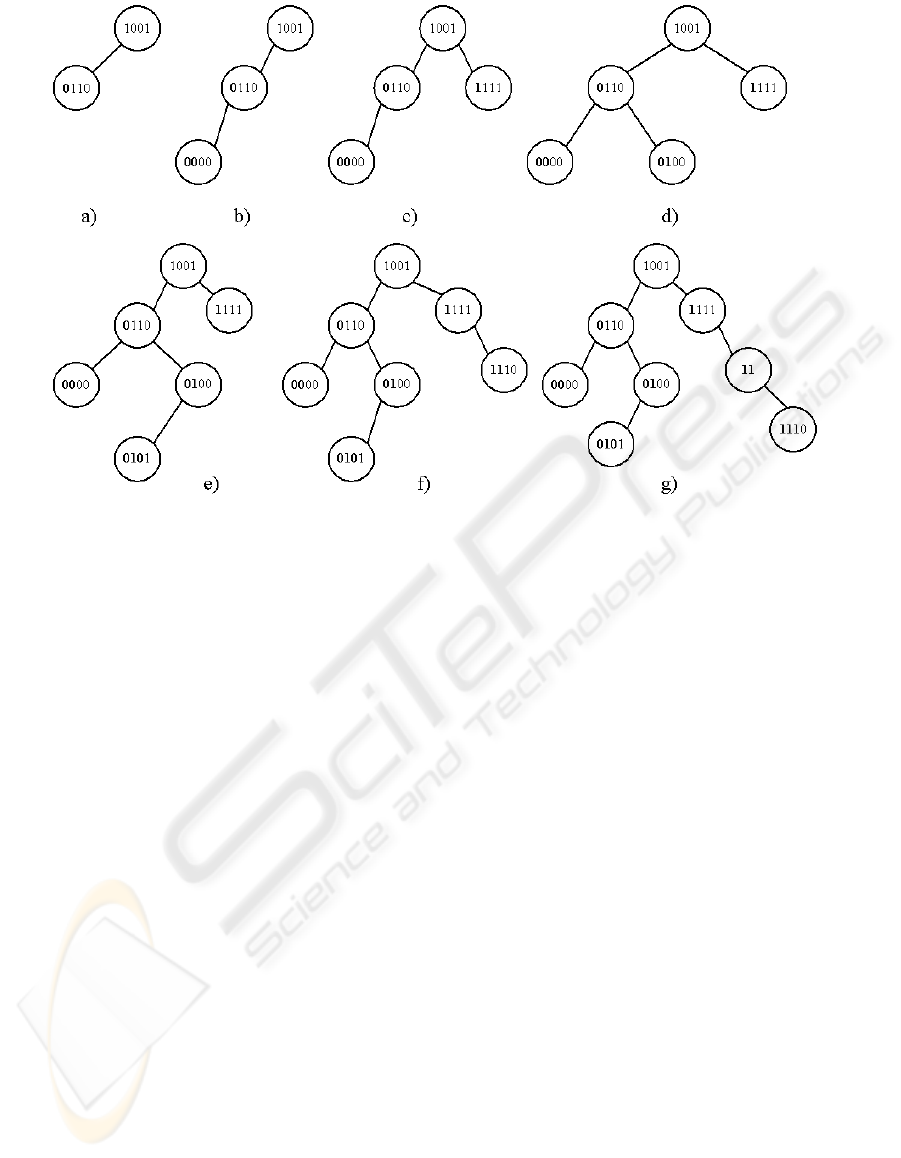
Figure 1: Creating a digital search tree.
means that the search key does not exist in the tree.
The above discussion deals with the case where
all keys are of equal length, which happens in many
applications (e.g. when the keys are integers). The al-
gorithm requires only a minor modification to handle
variable length keys. Consider, for example, how the
key 11 can be added to the tree in Figure 1f. As be-
fore, we follow the right link twice, because the first
two bits are 1. At this point we have run out of bits to
analyze. In such a case, it is obvious that the node we
are currently at has to have a key with a prefix equal
to the new key, and has to be longer than the new key
(otherwise the two keys are the same). Therefore, we
can place the new key (11) in place of the existing
node (1110), and continue by inserting the existing
node (1110) further down the tree. Since the third bit
of 1110 is 1, we go to the right, and place the new
node there because we have reached a NIL link. The
resulting tree is shown in Figure 1g.
Searching trees with keys of variable length is also
simple. If we run out of bits to analyze, the search
is terminated because the key sought does not exist
in the tree. The algorithms for dealing with keys of
variable length were originally presented in (Nebel,
1996).
2.2 Deleting Nodes From Dsts
Procedure to delete a node in the DST simply replaces
the node with any leaf node in either of the node’s
subtrees (E. Coffman, 1970). If the node to be deleted
does not have any children, it is simply removed and
replaced by a NIL pointer. For instance, removing the
node 0110 from the tree in Figure 1g can be done by
replacing it with either node 0000 or 0101. It is obvi-
ous that this method is similar, and in fact simpler than
the deletion method for ordinary binary trees, which
has to consider three distinct cases (Cormen, 1998)
2.3 Sorted Dsts
A DST is not a binary search tree, i.e. printing a DST
in-order will not produce a sorted sequence of tree’s
elements. This is not a major concern, because there
are many applications that do not require trees to be
sorted. However, algorithms for DSTs can be modi-
fied to produce a sorted digital search tree, providing
that all the keys are of the same length, and that the
key’s binary representation directly defines the order-
ing. This is the case for unsigned numbers, but not for
signed numbers. The most significant bit of a signed
number denotes the sign, and does not contribute to
the value according to its weight. Therefore, signed
numbers cannot be directly organized into a sorted
DST. Instead, two sorted DSTs could be created, one
for positive and one for negative numbers. Care must
be taken to order negative numbers appropriately.
Sorted DSTs can also be implemented when the
keys are strings of variable length, by padding all the
keys to the same length, either by explicitly padding
any unused characters with a terminating character
(’\0’ in C), or by constructing the algorithm to be-
ON DIGITAL SEARCH TREES - A Simple Method for Constructing Balanced Binary Trees
63

have as if the terminating characters were there. To
the best of our knowledge, no other publication has
discussed a technique to sort DSTs.
The following algorithm for constructing sorted
DSTs uses an idea similar to the one used in (Nebel,
1996). For the algorithm to work, the bits have to be
scanned from the most-significant to the least signifi-
cant as the tree is traversed. The procedure takes two
arguments, T and x, where T is a (possibly empty)
sorted DST, and x is a node to be inserted into the tree,
containing a key k
x
, and pointers left and right set to
NIL. It is assumed that the key k
x
can be represented
as a sequence of bits k
x
[n-1], k
x
[n-2],..., k
x
[0].
Algorithm 2.1: INSERT(T, x)
y ← root(T)
z ← NIL
i ← n
while y 6= NIL
do
i ← i− 1
c ← k
x
− k
y
if c = 0
then return
if (c > 0 and k
x
[i] = 0) or (c < 0 and k
x
[i] = 1)
then
temp ← k
y
k
y
← k
x
k
x
← temp
z ← y
if k
x
[i] = 0
then y ← left(y)
else y ← right(y)
if z = NIL
then root(T) ← x
else if k
x
[i] = 0
then left(z) ← x
else right(z) ← x
At each step down the tree, we analyze the corre-
sponding bit of k
x
to choose the appropriate path down
the tree and compare the new key k
x
with the current
key k
y
. If the corresponding bit is 0, and k
x
< k
y
, we
continue down the left branch, because this preserves
both the digital search tree structure and the binary
search tree structure. Conversely, if the correspond-
ing bit is 1 and k
x
> k
y
, we continue down the right
branch. However, if the corresponding bit is 0, and
k
x
> k
y
, it is impossible to satisfy both properties by
proceeding with the node x. Instead, we insert the
node x in place of the node y, and continue the inser-
tion down the left branch, now inserting the node y.
The node y has to go into the left branch, because k
y
is
lower than k
x
. Also, its corresponding bit has to be 0,
because the bits are ordered from the most significant
to the least significant, and since k
x
has the bit equal
to 0, and k
y
< k
x
, k
y
’s bit in the same position has to
be 0. This ensures that both the digital search tree and
the binary search tree structure is preserved. The pro-
cedure is similar when the corresponding bit of k
x
is
1, and k
x
< k
y
; we insert x in place of y, and proceed
down the right branch to insert y into an appropriate
spot. This process eventually terminates when a NIL
link is reached.
Sorted DSTs can be searched using the search pro-
cedure for either binary search trees or digital search
trees, because the sorted DSTs are binary search trees.
On the other hand, the delete procedure has to be con-
structed as follows. If a node x is to be deleted from
the tree, we locate the lowest element in the right sub-
tree (x’s successor), or the highest element in the left
subtree (x’s predecessor) if there is no right subtree.
Let us call that node d. We now move d in place of
x, and continue the process by deleting d from its old
place using the same procedure. The process termi-
nates once the selected node d does not have any chil-
dren, at which point its deletion is a trivial matter. We
can move d in place of x because d is either x
′
s prede-
cessor or successor, so the binary search tree structure
will be preserved. The digital search tree structure is
preserved because a node can be replaced by any of
its descendants, because they lie in the same subtree,
so the appropriate bits have to match (Knuth, 1997).
2.4 Properties of Digital Search Trees
The idea of DSTs can be extended to consider more
than one bit at a time. For instance, in an M-ary tree
(M ≥ 2), each node can have more than two chil-
dren (Knuth, 1997).
A DST with node keys of length |k| (|k| >0) has
the height h at most equal to |k| (Sedgewick, 1990).
Since all the algorithms described in the previous sec-
tions run in O(h) time, and the height of the tree is
limited by the binary length of the key |k|, all the al-
gorithms run in O(|k|) time in the worst case. On
average, if the keys are distributed uniformly across
all possible binary values, these algorithms require
O(log
2
n), according to (Sedgewick, 1990). For most
other tree data structures the worst-case performance
is expressed in terms of the number of elements in the
tree. For DSTs the worst case performance is given
in terms of the key length, so these expressions are
not directly comparable. Therefore, we believe that
experimental evaluation is the best way to compare
DSTs with other tree structures. We present our ex-
perimental evaluation in the following section.
3 EXPERIMENTAL EVALUATION
In this section we compare the effectiveness of digital
search trees, binary search trees, AVL trees and red-
black trees. To make the comparison fair, we used an
ICSOFT 2007 - International Conference on Software and Data Technologies
64

existing implementation of binary search trees, AVL
and red-black trees. We chose the GNU libavl (Pfaff,
2006) library of binary tree routines implemented in
C, because of its completeness and extensive docu-
mentation. The code for binary search trees, AVL and
red-black trees was used as provided in the library.
We used the code versions without parent pointers be-
cause they were not needed in any of our experiments.
DST code was based on the libavl code for binary
search trees. Only the necessary changes were made,
and all function prototypes were kept the same. In-
sert and search procedures for DSTs are very similar
to those for binary search trees; the only difference is
how the choice of the next direction down the tree is
made. As a consequence, only a few lines of code for
these methods differ between the binary search tree
and digital search tree implementation. For instance,
for trees that store integer key values, the source code
for the insert routine differs in only three lines of
code, while the search routine differs in five lines of
code.
In libavl, a node contains left and right pointers,
and a data pointer, which points to user data, in-
cluding the key. For the red-black and AVL trees,
each node also contains additional data (one charac-
ter) to implement balancing. We used this default
node structure in all our implementations, with the
data pointer pointing to the key. No other data was
stored in our experiments.
3.1 Experimental Setup
All program code is written in C, and compiled with
Microsoft’s 32-bit C/C++ Optimizing Compiler Ver-
sion 14.00.50727.42, which ships with the Microsoft
Visual C++ 2005 Express Edition. All programs were
compiled using the default settings for a Release ver-
sion (/02 optimization level).
The experiments described in this section were
run on a dedicated personal computer with Intel Pen-
tium 4 processor, with 8 Kbytes L1 cache and 512
Kbytes on-chip L2 cache, running at 2GHz, with 1GB
memory, and running Windows XP Professional Ver-
sion 2002, SP2. Each experiment was repeated five
times, and the average execution times are reported.
Two groups of experiments were performed. In
the first group of experiments integers were used as
keys in the binary tree, while character strings were
used in the second group. A summary of settings in
these experiments is given in Table 1. The columns
in the table indicate the data type used in different ex-
periments, and the order in which the elements were
inserted into the tree (random, ascending or descend-
ing). The ordering refers to the ordering of the keys.
Table 1: List of experiments performed.
Data type Ordering
Experiment Int String Rand. Asc. Desc.
I1 X X
I2 X X
I3 X X
S1 X X
S2 X X
S3 X X
S4 X X
Ordered insertion tests the performance of tree struc-
tures for the case that is normally the worst-case sce-
nario for the binary search trees.
In all experiments other than S4, the keys were
generated randomly, with uniform distribution, and
were all of equal length. For experiments I1-I3,
the number of elements in the tree was varied from
100,000 to 10,000,000, increasing the number of el-
ements 10 times in each experiment. For experi-
ments S1-S3, the number of elements was varied from
10,000 to 1,000,000 in the same manner. For these ex-
periments we also used three different string lengths:
12, 20 and 40 characters. However, since we did not
observe a significant variation in performance trends
for different string lengths, we present only the per-
formance results for strings of length 20.
In I1-I3 and S1-S3, two input files with mutually
disjoint key sets were used in each experiment. The
keys in the first file are used to create a binary tree,
and the time required to create the tree is measured.
All the keys were brought into a memory array be-
fore being added to the tree or any searches being
performed. Therefore, the reported execution times
do not include any disk accesses initiated by our pro-
grams.
Next, a search is performed for every key in the
first file, which verifies that all keys have been added
and can be located in the tree; search time is measured
and recorded. Then, a search for the keys in the first
file and the keys in the second file is performed. Since
the keys in these files are mutually disjoint, this mea-
sures the performance of searches when half the keys
sought do not exist in the tree. Next, a search for the
keys in the second file is performed, which provides
the execution time of searches for keys that do not ex-
ist. The keys in the second file were not sorted in any
of the experiments, which means that a search for the
elements was performed in random order.
Finally, the nodes in the tree are deleted, one by
one, in the same order they were inserted in. The time
for this operation is measured as well. To make sure
that the delete operation does not leave the tree un-
balanced, another experiment was performed, where
ON DIGITAL SEARCH TREES - A Simple Method for Constructing Balanced Binary Trees
65

a search for the keys from the first file is executed at
several checkpoints during the deletion process, and
the total search time is measured.
Experiment S4 stores a dictionary of strings of
variable length, with the maximal length of 24 char-
acters. The dictionary was The Gutenberg Webster’s
Unabridged Dictionary (Project Gutenberg, 2007)
with 109,327 words, 93,468 of which were unique.
Only the words, not their explanations, were added
to the tree. The second file was a novel (English
translation of Les Miserables, by Victor Hugo) down-
loaded from the same website, with 567,616 phrases,
489,431 of which were found in the dictionary. Ex-
periment S4 represents a near-worst-case for DSTs,
because the keys are of variable length, and many of
the keys are prefixes of other keys.
3.2 Search Tree Implementations
We implemented several different versions of the pro-
gram code. For DSTs storing integer keys, we used
three different versions: scanning bits from left to
right (most-significant to least-significant) while pro-
gressing down the tree (DSTL), scanning bits from
right to left (DSTR), and a sorted digital search tree
(DSTS). Performance of these variants is compared
to that of binary search trees (BST), AVL trees (AVL),
and red-black trees (RB).
For algorithms for storing strings we used libavl
implementation of binary search trees, AVL and red-
black trees. We only had to modify the comparison
function, which originally compared integers. We
used the standard C library strcmp function for this
purpose. We refer to these implementations as SBST,
SAVL and SRB to distinguish them from the corre-
sponding implementations using integer keys.
We also tested three different implementations of
DSTs storing character string keys. First, we used
a straightforward implementation, where individual
characters in a string are scanned in order, from left to
right, and analyzed bit-by-bit, also from left to right as
we progress down the tree. Keys of variable lengths
are handled using the algorithm described in (Nebel,
1996). We call this implementation SDSTC.
Next, we tried to optimize the performance by ob-
serving that most computers perform logical opera-
tions (such as bit extraction) on integers, not charac-
ters. Therefore, we can look at the string of characters
as an array of bits, which can be cast into an arbi-
trary data. We cast characters into integers, moving
along the character array from left to right, four char-
acters at a time. However, we scan the individual inte-
gers (after the cast) from right to left. This is because
the computer we ran the experiments on has the little-
endian memory organization, so this order of analyz-
ing bits corresponds well (though not completely) to
the ordinary left to right scanning order of SDSTC. In
this implementation we also cast characters into in-
tegers in the comparison function, which speeds up
the comparison, compared to the implementation us-
ing the strcmp function. The number of characters in
the string has to be divisible by 4 for this to be pos-
sible, which is not a severe limitation. We call this
implementation SDSTL.
Finally, we implemented a sorted version of dig-
ital search trees for strings. This implementation is
called SDSTS; it scans the input string character-by-
character from left to right to preserve ordering.
We observed that the keys being analyzed by the
algorithms share a common prefix with the key being
sought, inserted or deleted from the tree. This com-
mon prefix becomes longer as we progress down the
tree. Therefore, we can skip these bits when the al-
gorithms check for string equality. If this is done at
the character granularity (i.e. only skip 8, 16, 24,...
bits once that many tree levels have been traversed),
it is easy to implement and reduces the comparison
time. We call this technique reduced comparison.
This technique was employed for SDSTC and SDSTS
implementations, but not for SDSTL, because it is
more complicated to implement in that implementa-
tion, and does not benefit performance.
For SDSTL and SDSTS implementations, we pad
any unused characters with the terminating character
’\0. The padding is done at insertion time, as well
as when searching for or deleting a node. To make
the comparisons fair, we include the time to pad the
unused characters in our measurements.
3.3 Results
3.3.1 Average Node Depth and Tree Depth
Aside from execution time, we use two metrics to
evaluate different algorithms: average node depth and
tree depth. The average node depth is relevant be-
cause it determines the expected number of steps the
algorithms have to perform. The tree depth is defined
by the depth of the leaf with the greatest depth. There-
fore, it defines the worst case for operations on binary
trees.
The average node depths and tree depths for
various experiments relative to the performance of
AVL/SAVL tree are shown in tables 2 and 3. The re-
sults are averages over all tree sizes, because in most
cases the relative results do not differ much as the tree
size grows. For several experiments we do not give
values for BST/SBST, because not all experiments
ICSOFT 2007 - International Conference on Software and Data Technologies
66
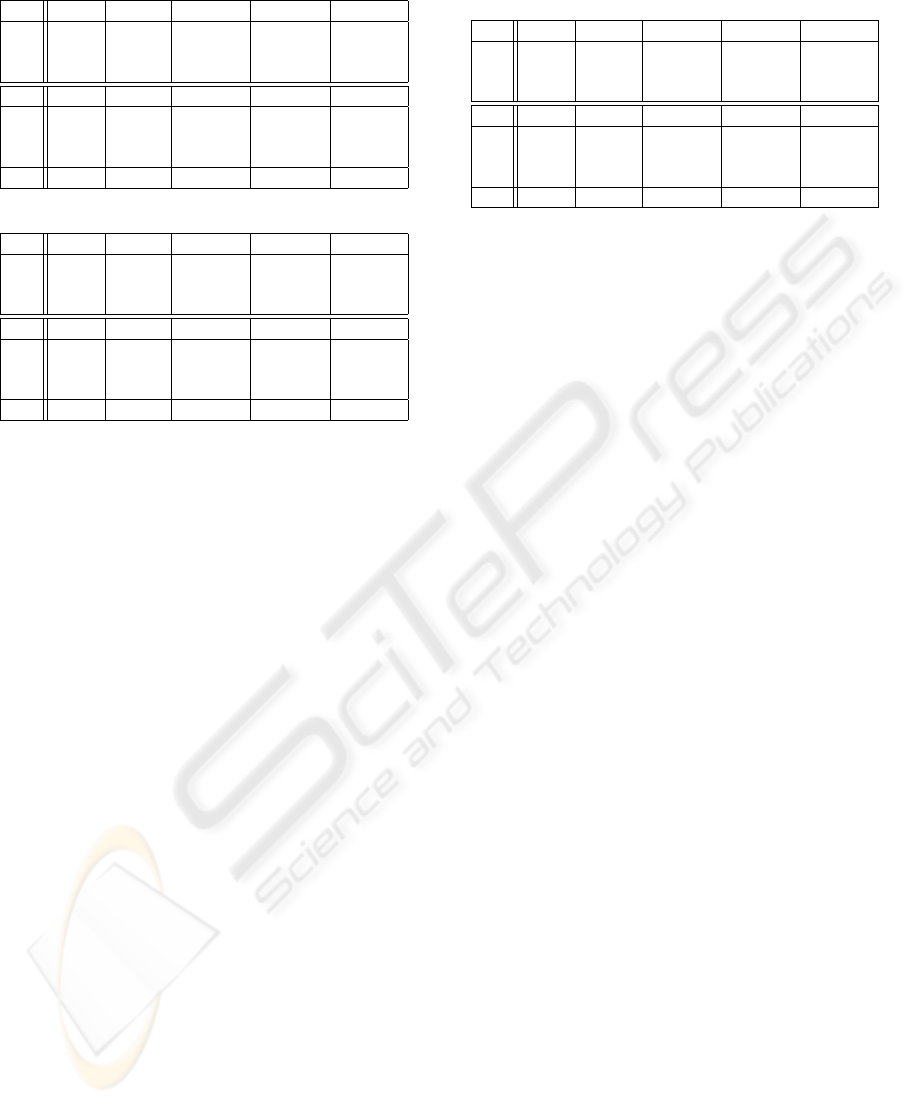
Table 2: Average node depth relative to AVL and SAVL.
RB BST DSTL DSTR DSTS
I1 1.00 1.34 1.01 1.00 1.01
I2 1.02 N/A 1.04 1.01 1.04
I3 1.02 N/A 1.04 1.01 1.04
SRB SBST SDSTL SDSTC SDSTS
S1 1.00 1.35 1.14 1.23 1.24
S2 1.03 N/A 1.16 1.27 1.26
S3 1.03 N/A 1.16 1.26 1.26
S4 1.00 889 2.17 2.38 2.39
Table 3: Tree depth relative to AVL and SAVL.
RB BST DSTL DSTR DSTS
I1 1.00 2.09 1.04 1.04 1.07
I2 1.88 N/A 1.31 1.24 1.30
I3 1.88 N/A 1.32 1.23 1.30
SRB SBST SDSTL SDSTC SDSTS
S1 1.00 1.97 1.20 1.29 1.29
S2 1.85 N/A 1.41 1.59 1.52
S3 1.85 N/A 1.44 1.57 1.52
S4 1.71 1443 4.35 4.47 4.76
with BSTs were completed because of excessive run-
time.
In experiments I2, I3, S2 and S3, the tree depth
of red-black trees is significantly higher than that of
AVL trees, which is expected, because the red-black
trees do not achieve as good balancing as the AVL
trees (Cormen, 1998). These results show that the
DSTs, including the sorted DSTs, do a good job of
keeping the tree balanced, with average node depth
comparable to that of AVL and red-black trees, and
tree depth between that of AVL and red-black trees,
for all but the last experiment (S4). Our experiments
showed that these large differences for S4 do not
translate into large performance differences.
3.3.2 Performance of the Insert Procedure
Table 4 presents the performance of the insert proce-
dure for the largest dataset in each experiment.
DSTL and SDSTL provide the best performance
in all cases except for S4. This was the case for all tree
sizes, although the ratio becomes smaller as the tree
size shrinks. (S)AVL and (S)RB exhibit poorer per-
formance because of complicated rotations they have
to perform to keep the tree balanced.
RB and DSTR give much lower relative perfor-
mance for experiments I2 and I3, which is surprising
considering that the tree depth and the average node
depth do not vary drastically for these experiments
(see tables 2 and 3). The reason is the effect proces-
sor caches have on performance; the other algorithms
experience improved performance due to cache local-
ity when the inputs are sorted, while RB and DSTR
do not. For example, for DSTL, where the bits are
Table 4: Insertion performance relative to AVL and SAVL
for largest datasets.
RB BST DSTL DSTR DSTS
I1 1.01 1.08 0.82 0.76 1.05
I2 3.00 N/A 0.89 4.19 0.94
I3 2.41 N/A 0.86 3.44 1.03
SRB SBST SDSTL SDSTC SDSTS
S1 1.04 1.11 0.65 0.82 1.00
S2 1.66 N/A 0.75 0.91 1.14
S3 1.65 N/A 0.76 0.91 1.11
S4 1.53 587 1.11 1.40 1.75
scanned from left to right, elements are repeatedly in-
serted into the same branch of the tree. This means
that the whole chain of pointers leading to the place
for a new node are already in the cache in many cases.
Since DSTR analyzes the bits from the right, where
the bits vary more often, it is likely to insert a new
element into a different branch of the tree most of the
time, so it has poor cache locality. Therefore, DSTR
is a poor choice for a scanning method and should not
be used.
The most interesting result is the one for experi-
ment S4. Although the three digital search trees have
an average node depth more than twice the depth of
the AVL trees, the SDSTL is only 11% slower than
SAVL, and faster than SRB. Even the straightforward
implementation, SDSTC, or the sorted version, SD-
STS, do not suffer performance penalties proportional
to the difference in node depth. This can be explained
through better utilization of cache locality. Digital
search trees exhibit better cache locality than the red-
black and AVL trees for two reasons. First, the nodes
in digital search trees are never (or only sometimes
for SDSTS) moved from their initial position, thereby
better preserving spatial locality. Also, the nodes in
digital search trees are smaller because they do not
include balancing information, so more can fit into a
cache. Consequently, a node and its children are more
likely to reside in the same cache line, thus improving
the performance. For these reasons, the digital search
trees are well suited for execution on modern com-
puters. Although other methods for exploiting cache
locality in binary trees exist (Oksanen, 1995), they ex-
plicitly manage memory allocation and/or tree struc-
ture, which makes the algorithms even more complex.
In contrast, digital search trees exhibit good locality
implicitly, based on their structure.
We have not shown the results for all tree sizes, but
the general trend is that the performance gap between
different algorithms, as presented in Table 4, tends to
grow linearly as the number of elements in the tree
grows exponentially.
ON DIGITAL SEARCH TREES - A Simple Method for Constructing Balanced Binary Trees
67
3.3.3 Search Performance
We do not present all the results for search routines
because they are similar to the results for the insert
routine. This is not surprising, because these two rou-
tines are similar in structure.
We observed a general trend that digital search
trees tend to perform better when fewer elements
sought are actually found in the tree. One interest-
ing case where this is particularly evident is experi-
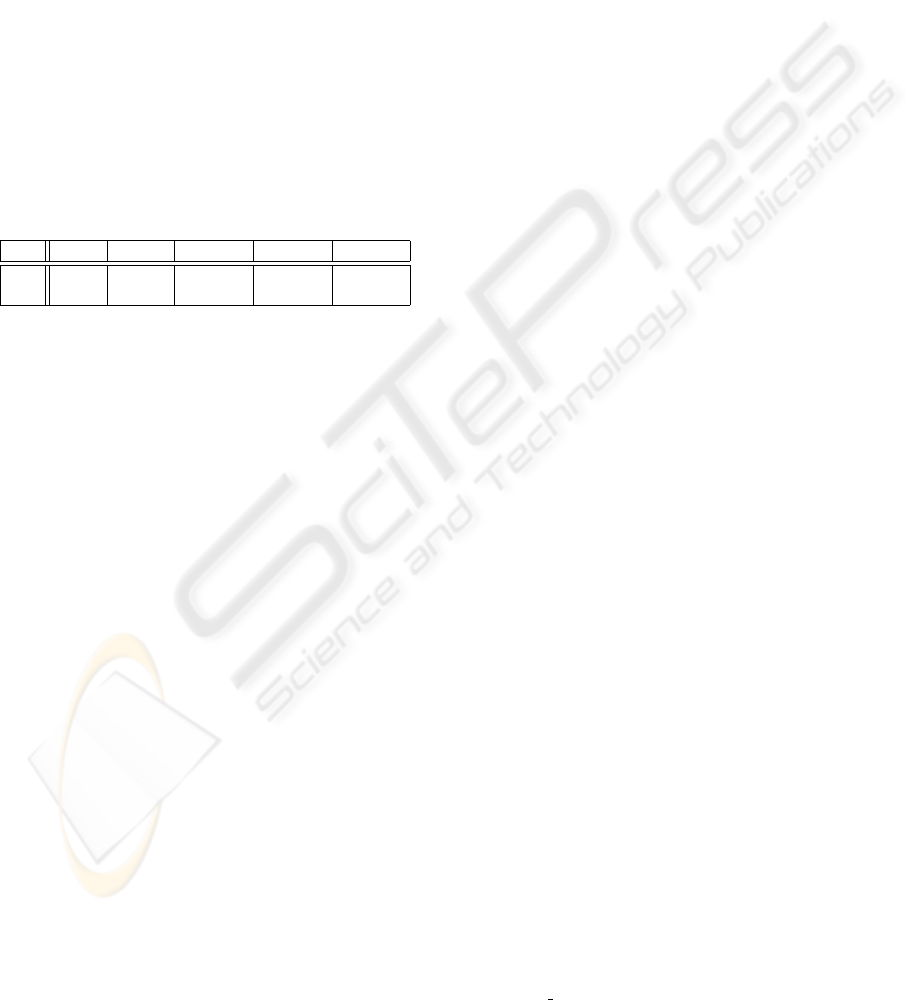
ment S4. Table 5 gives the performance results rel-
ative to SAVL, as the number of elements that were
actually found decreases. The FA and FS rows de-
note Found All and Found Some, respectively, and
correspond to searching for all the words in the dic-
tionary, and searching for the words from the book, as
described in section 3.1.
Table 5: Performance for two different searches in experi-
ment S4.
SRB SBST SDSTL SDSTC SDSTS
FA 1.01 960 1.39 1.95 2.24
FS 1.05 308 0.90 1.07 1.37
The FA search, in which all the elements sought
are found, is the worst case we found for the digital
search trees. Even then, only the sorted (SDSTS) and
the straightforward implementation (SDSTC) suffer
penalties proportional to the average node depth. A
more clever implementation, SDSTL, which is still
much simpler to implement than the other balanced
tree algorithms, suffers a modest penalty of 39% in
the worst case. When the elements sought are found
less often, the relative performance of all DST trees
improves significantly.
3.3.4 Delete Performance
We do not present the results for delete routines for
experiments I1-I3 and S1-S3, because they show sim-
ilar trends as the insert routine. For the experiment
S4, we found that SRB, SDSTL, SDSTC and SDSTS
have 15%, 46%, 69%, and 34% worse performance
than SAVL, respectively. At the same time, SBST
performs 12% better than SAVL when deleting the
nodes.
We also checked the search performance at sev-
eral checkpoints throughout the deletion process, and
found that SRB, SDSTL, SDSTC and SDSTS achieve
6%, 20%, 59%, and 79% worse search performance
than SAVL, respectively. SBST takes 180 times
longer than SAVL in this case. These results resemble
the search performance in Table 5.
4 CONCLUSIONS
We discussed the digital search trees (DSTs), which
use the values of bits in the key to determine the key’s
position in the tree. We believe that these trees are
easier to understand conceptually, and easier to im-
plement in practice than other known balanced trees.
We found that only small modifications to algorithms
for ordinary binary search trees are needed to imple-
ment the digital search trees.
Our experiments show that performance of digi-
tal search trees is often as good or better than AVL or
red-black trees. The digital search trees can be rec-
ommended for use whenever the keys stored are in-
tegers, or character strings of fixed width. We found
that these trees are also suitable in many cases when
the keys are strings of variable length.
We believe that these trees deserve renewed atten-
tion. Novel techniques may be discovered that im-
prove the performance even further. Also, new ap-
plications may be discovered that could benefit from
using the digital search tree as a data structure.
REFERENCES
Andersson, A. (1993). Balanced search trees made sim-
ple. In WADS, 3rd Workshop on Algorithms and Data
Structures, pages 60–71. Springer Verlag.
Cormen, T. H. (1998). Introduction to Algorithms. MIT
Press, Cambridge, Mass, 2nd edition.
E. Coffman, J. E. (1970). File structures using hashing func-
tions. Communications of the ACM, 13(7).
F. Flajolet, R. S. (1986). Digital search trees revisited. SIAM
Journal on Computing, 15(3).
Knuth, D. E. (1997). The Art of Computer Programming,
volume 3. Addison-Wesley, Reading, Mass., 2nd edi-
tion.
Nebel, M. E. (1996). Digital search trees with keys of vari-
able length. Informatique Theorique et Applications,
30(6):507–520.
Oksanen, K. (1995). Memory Reference Locality in Binary
Search Trees. Master’s thesis, Helsinki University of
Technology.
Pfaff, B. (2006). Gnu libavl. http://adtinfo.org.
Project Gutenberg (2007). The Guten-
berg Webster’s unabridged dictionary.
http://www.gutenberg.org/etext/673.
Sedgewick, R. (1990). Algorithms in C. Addison-Wesley,
Reading, Mass.; Toronto.
Wikipedia, The Free Encyclopedia
(2007). Category:trees(structure).
http://en.wikipedia.org/wiki/Category:
Trees
%28structure%29.
ICSOFT 2007 - International Conference on Software and Data Technologies
68
