MODERN CONCEPTS FOR

HIGH-PERFOMANCE SCIENTIFIC COMPUTING

Library Centric Application Design

Ren

e Heinzl, Philipp Schwaha and Siegfried Selberherr

Institute for Microelectronics, TU Wien, Gusshausstrasse 27-29, Vienna, Austria

Keywords:

Scientiﬁc computing, high performance computing, concept based programming, multi paradigms, partial

differential equations.

Abstract:

During the last decades various high-performance libraries were developed written in fairly low level lan-

guages, like FORTRAN, carefully specializing codes to achieve the best performance. However, the objective

to achieve reusable components has been regularly eluded by the software community ever since. The funda-

mental goal of our approach is to create a high-performance mathematical framework with reusable domain-

speciﬁc abstractions which are close to the mathematical notations to describe many problems in scientiﬁc

computing. Interoperability driven by strong theoretical derivations of mathematical concepts is another im-

portant goal of our approach.

1 INTRODUCTION

This work reviews common concepts for scientiﬁc

computing and introduces new ones for a timely ap-

proach to library centric application design.

Based on concepts for generic programming, e.g.

in C++, we have investigated and developed data

structures for scientiﬁc computing. The Boost Graph

Library (Siek et al., 2002) was one of the ﬁrst generic

libraries, which introduced concept based program-

ming for a more complex data structure, a graph. The

actual implementation of the Boost Graph Library

(BGL) is for our work of secondary importance, how-

ever, we value the consistent interfaces for graph op-

erations. We have extended this type of concept based

programming and library development to the ﬁeld of

scientiﬁc computing. To give a brief introduction we

use an example resulting from a self-adjoint partial

differential equation (PDE), namely the Poisson equa-

tion:

div(ε grad(Ψ)) = ρ

Several discretization schemes are available to

project this PDE into a ﬁnite space. We use the

method of ﬁnite volumes (FV (Selberherr, 1984)).The

resulting equations are given next, where A

and d

represents geometrical properties of the discretized

space, ρ the space charge, Ψ the potential, and ε the

permittivity of the medium.

∑

= ρ (1)

− Ψ

+ ε

(2)

An example of our domain speciﬁc notation is

given in the following code snippet and explained in

Section 4:

value =

(

sum<vertex_edge >

[

diff<edge_vertex >

[

Psi(_1)

] * A(_1)/d(_1) *

sum<edge_vertex >[eps(_1)]/2

] - rho(_1)

)(vertex);

Generic Poisson Equation

As can be seen, the actual notation does not de-

pend on any dimension or topological type of the cell

100

Heinzl R., Schwaha P. and Selberherr S. (2007).

MODERN CONCEPTS FOR HIGH-PERFOMANCE SCIENTIFIC COMPUTING - Library Centric Application Design.

In Proceedings of the Second International Conference on Software and Data Technologies - SE, pages 100-107

DOI: 10.5220/0001327401000107

 SciTePress

complex (mesh) and is therefore dimensionally and

topologically indepent. Only the relevant concepts,

in this case, the existence of edges incident to a ver-

tex and several quantity accessors, have to be met. In

other words, we have extended the concept program-

ming of the standard template library (STL) and the

generic programming of C++ to higher dimensional

data structures and automatic quantity access mecha-

nisms.

Compared to the reviewed related work given in

Section 2, our approach implements a domain spe-

ciﬁc embedded language. The related topological

concepts are given in Section 3, whereas Section 4

brieﬂy overviews the used programming paradigms.

In Section 5 several application examples are pre-

sented. The ﬁrst example introduces a problem of

a biological system with a simple PDE. The second

example shows a nonlinear system of coupled PDEs,

which makes use of the linearization framework intro-

duced in Section 4.1, where derivatives are calculated

automatically.

For a successful treatment of a domain speciﬁc

embedded notation several programming paradigms

are used. By object-oriented programming the ap-

propriate iterators are generated, hidden in this exam-

ple in the expression

vertex edge

and

edge vertex

Functional programming supplies the higher order

function expression between the

[

and

]

and the un-

named function object

. And ﬁnally the generic pro-

gramming paradigm (in C++ realized with parametric

polymorphism or templates) connects the various data

types of the iterators and quantity accessors.

A signiﬁcant target of this work is the separa-

tion of data access and traversal by means of the

mathematical concept of ﬁber bundles (Butler and

Bryson, 1992). The related formal introduction en-

ables a clean separation of the internal combinatorial

properties of data structures and the mechanisms of

data access. A high degree of interoperability can be

achieved with this formal interface. Due to space con-

straints the performance analysis is omitted and we

refer to a recent work (Heinzl et al., 2006a) where the

overall high performance is presented in more detail.

2 RELATED WORK

In the following several related works are presented.

All of these software libraries are a great achievement

in the various ﬁelds of scientiﬁc computing.

The FEniCS project (Logg et al., 2003), which is

a uniﬁed framework for several tasks in the area of

scientiﬁc computing, is a great step towards generic

modules for scientiﬁc computing.

Femster (Castillo et al., 2005) is a class library

for ﬁnite element (FE) calculations. This means that

users must provide their own code for assembling

global FE matrices. In other words, Femster imple-

ments a general ﬁnite element API.

The Template Numerical Toolkit (Pozo, 1997)

is a collection of interfaces and reference implemen-

tations of numerical objects (matrices) in C++. The

toolkit deﬁnes interfaces for basic data structures,

such as multidimensional arrays and sparse matrices,

commonly used in numerical applications.

The Boost Graph Library is a generic interface

which enables access to a graph’s structure, but hides

the details of the actual implementation. All libraries

which implement this type of interface are interoper-

able with the BGL generic algorithms. This approach

was one of the ﬁrst in the ﬁeld of non-trivial data

structures with respect to interoperability. The prop-

erty map concept (Siek et al., 2002) was introduced

and heavily used.

The Grid Algorithms Library, GrAL (Berti,

2000) was one of the ﬁrst contributions to the uni-

ﬁcation of data structures of arbitrary dimension for

the ﬁeld of scientiﬁc computing. A common interface

for grids with a dimensionally and topologically inde-

pendent way of access and traversal was designed.

Our approach, the Generic Scientiﬁc Simulation

Environment, GSSE (Heinzl et al., 2006b) deals with

various modules for different discretization schemes

such as ﬁnite elements and ﬁnite differences. In

comparison, our approach focuses more on providing

building blocks for scientiﬁc computing, especially an

embedded domain language to express mathematical

dependencies directly, not only for ﬁnite elements.

To achieve interoperability between different li-

brary approaches we use concepts of the ﬁber bun-

dle theory to separate the base space and ﬁber space

properties. With this separation we can use several

other libraries (see Section 3) for different tasks. The

theory of ﬁber bundles separates the data structural

components from data access (ﬁbers). We have de-

veloped a consistent data structure interface for all

different types of data structures and several other li-

braries employing the theory of CW-complexes and

poset theory. Based on this interface speciﬁcation we

can use several libraries, such as STL, BGL, GrAL,

and accomplish high interoperability and code reuse.

3 CONCEPTS

Our approach extends the concept based program-

ming of the STL to arbitrary dimensions similar to

GrAL. The main difference to GrAL is the introduc-

MODERN CONCEPTS FOR HIGH-PERFOMANCE SCIENTIFIC COMPUTING - Library Centric Application Design

101

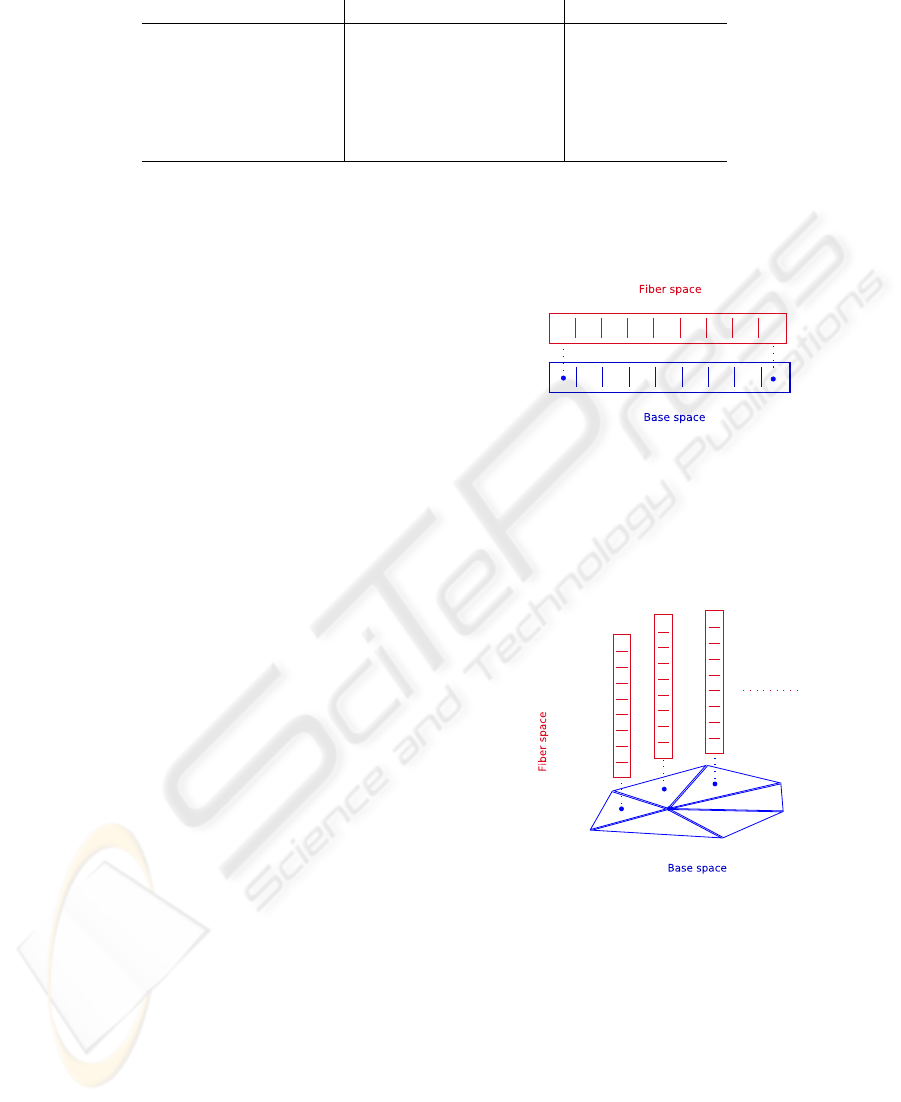
Table 1: Comparison of the cursor/property map and the ﬁber bundle concept.

cursor and property map ﬁber bundles

isomorphic base space no yes

traversal possibilities

STL iteration cell complex

traversal base space

yes yes

traversal ﬁber space

no yes

data access

single data topological space

ﬁber space slices

no yes

tion of the concept of ﬁber bundles, which separates

the base mechanism of application design into base

and ﬁber space properties. The base space is modeled

by a CW-complex and algebraic topology, whereas

the ﬁber space is modeled by a generic data accessor

mechanism, similar to the cursor and property map

concept (Abrahams et al., 2003).

3.1 Theory of Fiber Bundles

We introduce concepts of ﬁber bundles as a descrip-

tion for data structures of various dimensions and

topological properties.

• Base space: topology and partially ordered sets

• Fiber space: matrix and tensor handling

Based on these examples, we introduce a com-

mon theory for the separation of the topological struc-

ture and the attached data. The original contribu-

tion of this theory was given in Butler’s vector bun-

dle model (Butler and Bryson, 1992), which we com-

pactly review here:

Deﬁnition 1 (Fiber Bundle) Let E,B be topological

spaces and f : E → B a continuous map. Then

(E,B, f) is called a ﬁber bundle, if there exists a

space F such that the union of the inverse images of

the projection map f (the ﬁbers) of a neighborhood

⊂ B of each point b ∈ B are homeomorphic to

× F, whereby this homeomorphism has to be such

that the projection pr

of U

× F (that maps each el-

ement of this product space to the element of the ﬁrst

space) yields U

again.

E is called the total space, B is called the base space,

and F is called the ﬁber space. This deﬁnition re-

quires that a total space E can locally be written as

the product of a base space B and a ﬁber space F.

The decomposition of the base space is mod-

eled by an identiﬁcation of data structures by a CW-

complex. (Benger, 2004; Heinzl et al., 2006c). As an

example Figure 2 depicts an array data structure based

on the concept of a ﬁber bundle. We have a simple

ﬁber space attached to each cell (marked with a dot in

the ﬁgure), which conserves the neighborhood of our

base space and carries the data of our array.

Figure 2: A ﬁber bundle with a ﬁber space over a 0-cell

complex. A simple array is an example of this type of ﬁber

space.

The next ﬁgure depicts a ﬁber bundle with a 2-

cell complex as base space. For the base space of

Figure 3: A ﬁber space over a 2-simplex cell complex base

space. An example of this type of ﬁber space is a triangle

mesh with an array over each triangle.

lower dimensional data structures, such as an array or

single linked list, the only relevant information is the

number of elements determined by the index space.

Therefore most of the data structures do not separate

these two spaces. For backward compatibility with

common data structures the concept of an index space

depth is used (Heinzl et al., 2006c).

The advantages of this approach are similar to

those of the cursor and property map (Abrahams et al.,

2003), but they differ in several details. The similar-

ICSOFT 2007 - International Conference on Software and Data Technologies

102

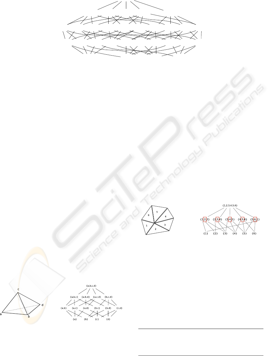
{0,1,2,3,4}

{0,1,2,3}

{0,1,2,4} {0,1,3,4}{0,2,3,4} {1,2,3,4}

{0,1,2} {0,1,3}{0,2,3} {1,2,3}{0,1,4}{0,2,4} {1,2,4}{0,3,4} {1,3,4}{2,3,4}

{0,1}{0,2} {1,2}{0,3} {1,3}{2,3}{0,4} {1,4}{2,4}

{0} {1}{2}

{3,4}

{3} {4}

Figure 1: Cell topology of a simplex cell in four dimensions.

ity is that both properties can be implemented inde-

pendently. However, the ﬁber bundle approach equips

the ﬁber space with more structure, e.g., storing more

than one value corresponding to the traversal position

as well as preservation of neighborhoods. This feature

is especially useful in the area of scientiﬁc computing,

where different data sets have to be managed, e.g.,

multiple scalar or vector values on vertices, faces, or

cells. Another important property of the ﬁber bundle

approach is that an equal (isomorphic) base space can

be exchanged with another cell complex of the same

dimension. Table 1 summarizes the common features

and the differences.

As can be seen the concept of the cursor and prop-

erty map can be extended to the ﬁber bundle approach

with additional properties and mechanisms.

3.2 Topological Interface

We brieﬂy introduce parts of the interface speciﬁca-

tion for data structures and their corresponding itera-

tion mechanism based on algebraic topology. A full

reference can be found in (Heinzl et al., 2006c). With

the concept of partial ordered sets and a Hasse dia-

gram we can order and depict the structure of a cell.

As an example the topological structure of a three-

dimensional simplex is given in Figure 4. Inter-

Figure 4: Cell topology of a 3-simplex cell.

dimensional objects such as edges and facets and their

relations within the cell can thereby identiﬁed. The

complete traversal of all different objects is deter-

mined by this structure. We can derive the vertex on

edge, vertex on cell, as well as edge on cell traver-

sal up to the dimension of the cell in this way. Based

on our topological speciﬁcation arbitrary dimensional

cells can be easily used and traversed in the same way

as all other cell types, e.g., a 4-dimensional simplex

shown in Figure 1.

Next to the cell topology a separate complex

topology is derived to enable an efﬁcient implemen-

tation of these two concepts. A signiﬁcant amount of

code can be reduced with this separation. Figure 5 de-

picts the complex topology of a 2-simplex cell com-

plex where the bottom sets on the right-hand sides are

now the cells. The rectangle in the ﬁgure marks the

relevant cell number. The topology of the cell com-

Figure 5: Complex topology of a simplex cell complex.

plex is only available locally because of the fact that

subsets can have an arbitrary number of elements. In

other words, there can be an arbitrary number of trian-

gles attached to the innermost vertex. Our ﬁnal classi-

ﬁcation scheme uses the term

local

to represent this

fact.

A formal concise deﬁnition of data structures can

therewith be derived and is presented in Figure 2. The

complex topology uses the number of elements of the

corresponding subsets.

complex_t <cells_t ,global > cx; //{1}

complex_t <cells_t ,local<2>> cx; //{2}

complex_t <cells_t ,local<3>> cx; //{3}

complex_t <cells_t ,local<4>> cx; //{4}

STL Data Structure Deﬁnitions

MODERN CONCEPTS FOR HIGH-PERFOMANCE SCIENTIFIC COMPUTING - Library Centric Application Design

103

Table 2: Classiﬁcation scheme based on the dimension of cells, the cell topology, and the complex topology.

data structure

cell dimension cell topology complex topology

array/vector 0 simplex global

SLL/stream

0 simplex local(2)

DLL/binary tree

0 simplex local(3)

arbitrary tree

0 simplex local(4)

graph

1 simplex local

grid

2,3,4,.. cuboid global

mesh

2,3,4,.. simplex local

Here {

} describes an array, {

} a stream or a sin-

gle linked list, {

} a doubly linked list or a binary

tree, and ﬁnally {

} an arbitrary tree. To demonstrate

the equivalence of the STL data structures and our ap-

proach we present a simple code snippet (the typedefs

are omitted due to space constraints):

cell_t <0, simplex> cells_t;

complex_t <cells_t , global > complex_t;

long

data_t;

container_t <complex_t , data_t >

container;

// is equivalent to

std::vector <data_t> container;

Equivalence of Data Structures

The separation of the topological structure and the

data speciﬁcation can be seen clearly here.

3.3 Data Access

In the following code snippet a simple example of the

generic use of a data accessor similar to the property

map concept is given, where a scalar value is assigned

to each vertex. The data accessor implementation

also takes care of accessing data sets with different

data locality, e.g., data on vertices, edges, facets, or

cells. The data accessor is extracted from the con-

tainer to enable a functional access mechanism with a

key value which can be modeled by arbitrary compa-

rable data types.

da_type da(container , key_d);

for_each(container.vertex_begin(),

container.vertex_end(),

da = 1.0 );

Data Accessor

Several programming paradigms are used in this

example which are presented in detail in the next sec-

tion, especially the functional programming, given in

this example with the

da = 1.0

4 PROGRAMMING PARADIGMS

Various areas of scientiﬁc computing encourage dif-

ferent programming techniques, even demands for

several programming paradigms can be observed:

• Object-oriented programming: the close interac-

tion of content and functions is one of the most

important advantages of the object-oriented pro-

gramming

• Functional programming: offers a clear notation,

is side-effect free and inherent parallel

• Generic programming: can be seen as the glue

between object-oriented and functional program-

ming

Our implementation language of choice is C++

due to the fact, that it is one of the few programming

languages where high performance can be achieved

with various paradigms. To give an example of this

multi-paradigm approach, a simple C++ source snip-

pet is given next.

std::for_each(v.begin(),v.end(),

if_(arg1 > 5)

[

std::cout << arg1 << std::cout

]

);

Multiple Paradigms

The object-oriented programming paradigm is used to

create the iterator capabilities of the container struc-

tures of the STL. This paradigm is not used anywhere

else in our approach. Functional programming is used

to create function objects which are passed into the

generic

for each

algorithm. In this example the no-

tation of the Boost Phoenix 2 (Pho, 2006) library is

used to create a functional object context, marked by

the

[

and

]

. The generic paradigm uses the template

mechanism of C++ to bind these two paradigms to-

gether efﬁciently. A more complex example is given

in the following expression. Here a cell complex of

arbitrary dimension is used and the vertex to vertex

iteration is expressed.

ICSOFT 2007 - International Conference on Software and Data Technologies

104

gsse::for_each((*segit).vertex_begin(),

(*segit).vertex_end(),

result=gsse::add<vertex_vertex >

(

_1+_2

)[quan]

);

Complex Functor

The same paradigms as in the example before can

be seen, but in this case, a complex topological traver-

sal is used instead of simple container traversal. The

topological properties of the GSSE are demonstrated

twofold: on the one hand side, the topological concept

programming allows the implementation of a dimen-

sionally independend algorithm. On the other hand

side, different data structures of library approaches

can be used, which fullﬁll the basic requirements of

the required topological concept. In this example all

data structures or libraries which implement means

of vertex to vertex traversal can be used. The func-

tional expression is also more complex and based on

the algebraic property of the identity element for the

gsse::add

operation as the initial value of the opera-

tion, in this case

. This GSSE algorithm sums up the

potential values of all adjacent vertices to a vertex.

The data accessor

quan

handles the storage mecha-

nism for the value attached to a vertex. Here the inter-

action of programming paradigms related to the base

space and ﬁber space can be seen clearly. The base

space traversal is built with the generic programming

paradigm, whereas the ﬁber space operation is imple-

mented by means of functional programming.

A lot of difﬁculties with conventional program-

ming can be circumvented by this approach. Func-

tional programming enables great extensibility due

to the modular nature of function objects. Generic

programming and the corresponding template mech-

anisms of C++ offer an overall high performance. In

addition arbitrary data structures of arbitrary dimen-

sions can be used. The only requirement is that the

data structure models the required concept, in this

case a vertex to vertex information.

4.1 Automatic Linearization

We introduce a calculation framework where deriva-

tives are implicitly available and do not have to be

speciﬁed explicitly. This enables the speciﬁcation of

nonlinear differential equations in a convenient way.

The elements of the framework are truncated Taylor

series of the following form f

∑

· ∆x

. To use

a quantity x

within a formula we have to specify its

value f

and the linear dependence c

= 1 on the vec-

tor x of quantities. This step, however, can be per-

formed implicitly by the computer. This non-trivial

and highly complex scenario yields itself exception-

ally well to the application of the functional program-

ming paradigm. In general, all discretization schemes

which use line-wise assembly based on ﬁnite differ-

ences as well as ﬁnite volumes can be handled with

the described formalism.

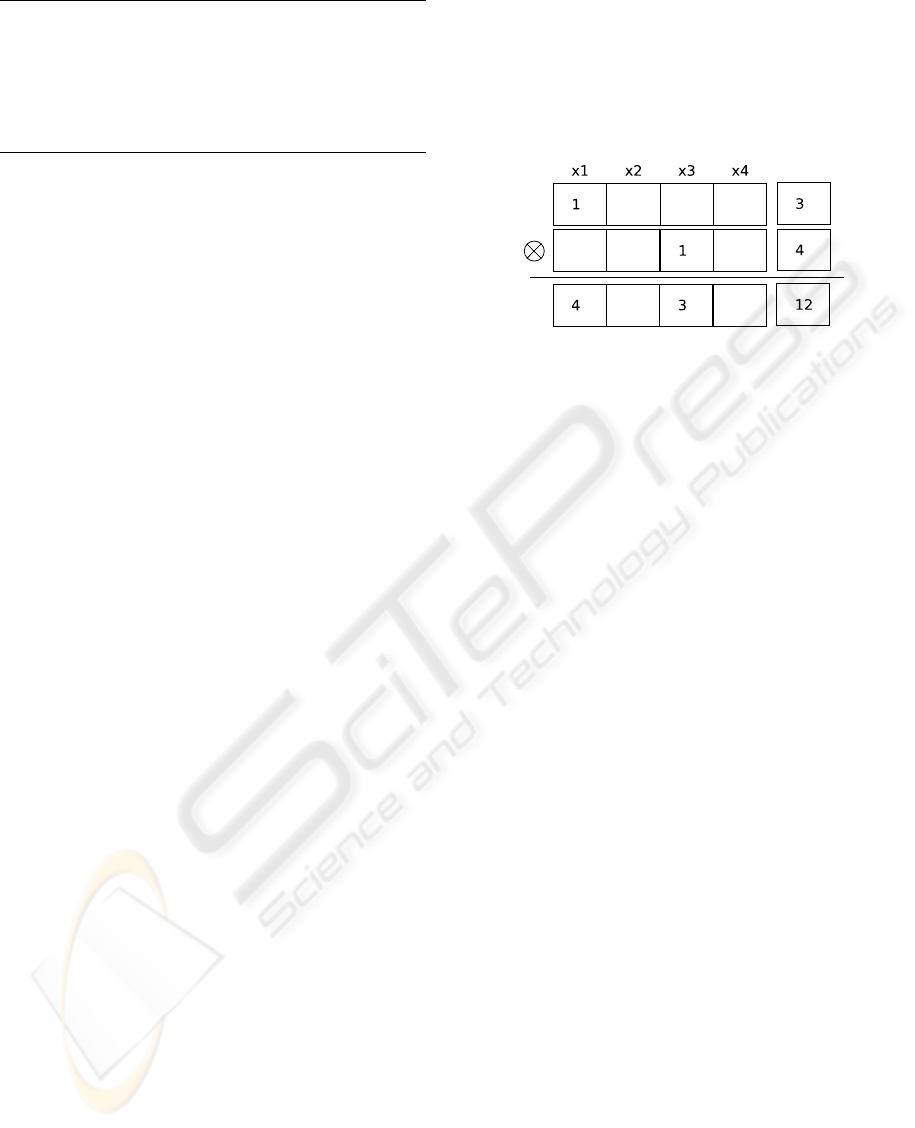
Figure 6: The multiplication of two Taylor series.

Basic operations on Taylor series can handle trun-

cated polynomial expansions. In the following we

specify our nonlinear functionals using linearized

functions in upper case letters. All necessary numer-

ical operations on these data structures can be per-

formed in a straight forward manner.

F = f

∑

· ∆x

, G = g

∑

· ∆x

(3)

F ⊕ G = ( f

+ g

) +

∑

+ d

) · ∆x

(4)

F ⊗ G = ( f

· g

) +

∑

· d

+ f

· c

) · ∆x

(5)

Having implemented these schemes we are able

to derive all required functions on these mathematical

structures. This means that we have a consistent

framework for formulas in the following sense: if A is

the linearized version of function

A at x

, we obtain

∂A/∂

= ∂

A /∂

around the point of linearization.

Figure 6 shows the multiplication of two truncated

expansions F = 3+ ∆x

, and G = 3+ ∆x

. As a re-

sult we obtain F ⊗ G = 12 + 4∆x

+ 3∆x

. By im-

plementing only the linear (or higher order polyno-

mial) functional dependence of equations on variables

around x we reduce the external speciﬁcation effort

to a minimum. Thus, it is possible to ease the spec-

iﬁcation with the functional programming approach,

while also providing the functional dependence of

formulas.

5 APPLICATION DESIGN

In the following we brieﬂy review a few applications

based on the introduced concepts with their respective

paradigms.

MODERN CONCEPTS FOR HIGH-PERFOMANCE SCIENTIFIC COMPUTING - Library Centric Application Design

105

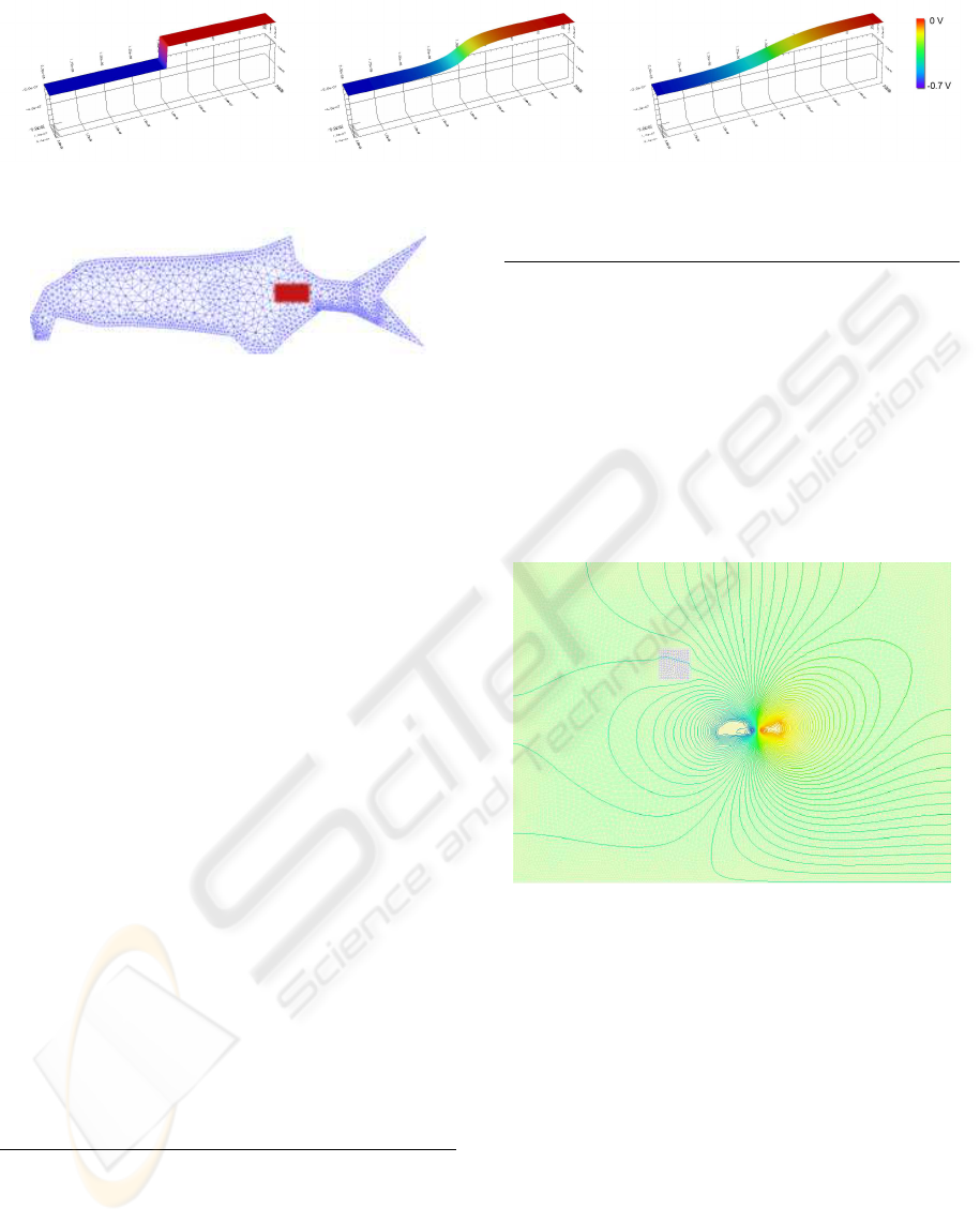
Figure 8: Potential in a pn diode during different stages of the Newton iteration. From initial (left) to the ﬁnal result(right).

Figure 7: Discretized domain of a ﬁsh with a red marked

electrically active organ.

5.1 Biological System

Electric phenomena are common in biological organ-

isms such as the discharges within the nervous sys-

tem, but usually remain within a small scale. In some

organisms, however, the electric phenomena take a

more prominent role. Some ﬁsh species, such as

Gnathonemus petersii from the family of Mormyridae

(Westheide and Rieger, 2003), use them for detection

of their prey. The up to 30 cm long ﬁsh actively gener-

ates electric pulses with an organ located near its tail

ﬁn (also marked in Figure 7). More information can

be found in (Schwaha et al., 2007).

For this case we derive the equation system based

on a quasi-electro-statical system directly from the

corresponding Maxwell equations. The charge sep-

aration of the electrically active organ which is ac-

tively taking place within parts of the simulation do-

main also has to be taken into account. We use the

conservation law of charge and the divergence theo-

rem (Gauss’s law) and ﬁnally get:

∂

[div(ε grad(Ψ))] + div(γ grad(Ψ)) = P (6)

Equation 6 is discretized using the ﬁnite volume dis-

cretization scheme. The high semantic level of the

speciﬁcation is illustrated by the following snippet of

code:

equation=sum<vertex_edge >(_v)

[

Orient(_v,_1) *

sum<edge_vertex >(_e)

[

lineqn(pot(_1), psi(_1))*Orient(_e,_1)

]

*(area(_1) / dist(_1))

*(gamma(_1)*deltat + eps(_1))

]+vol(_1)*((P(_1)*deltat)+rho(_1)))

This source snippets presents most of the applica-

tion code which has to be developed. In addition, only

a simple preprocessing step which creates the neces-

sary quantity accessors is required.

The simulation domain is divided into several

parts including the ﬁsh itself, its skin, that serves as

insulation, the water the ﬁsh lives in, and an object,

that represents either an inanimate object or prey. The

parameters of each part can be adjusted separately. A

result of the simulation is depicted in the following

ﬁgure:

Figure 9: Result of a simulation with a complete domain,

the ﬁsh, and a ideally conductor as response object.

5.2 Drift-Diffusion Equation

Semiconductor devices have become an ubiquitous

commodity and people expect a constant increase of

device performance at higher integration densities and

falling prices.

To demonstrate the importance of a method for

device simulation that is both easy and efﬁcient we

review the drift diffusion model that can be derived

from Boltzmann’s equation for electron transport by

applying the method of moments (Selberherr, 1984).

Note that this problem is a nonlinear coupled sys-

tem of partial differential equations where our lin-

earization framework is used. This results in current

ICSOFT 2007 - International Conference on Software and Data Technologies

106

relations as shown in Equation 7. These equations

are solved self consistently with Poisson’s equation,

given in Equation 8.

= qnµ

grad Ψ+ qD

grad n (7)

div(grad(ε Ψ)) = −ρ (8)

The following source code results from an application

of the ﬁnite volume discretization scheme:

linearequ_t equ_pot, equ_n;

equ_pot = (sum<vertex_edge >

[

diff<edge_vertex >[pot_quan]

] + ( n_quan - p_quan + nA - nD ) *

vol * q / (eps0 * epsr)

)(vertex);

equ_n = (sum<vertex_edge >

[

diff<edge_vertex >

( -n_quan*Bern(

diff<edge_vertex >[pot_quan /U_th]

-n_quan*Bern(

diff<edge_vertex >[-pot_quan/U_th]

)

)* (q * mu_h * U_th)

])(vertex);

Drift-Diffusion Equation

To brieﬂy present a simulation result we provide

Figure 8 which shows the potential in a pn diode

at different stages of a nonlinear solving procedure.

The leftmost ﬁgure shows the initial solution, while

the rightmost depicts the ﬁnal solution. The center

image shows an intermediate result that has not yet

fully converged. The visualization of the calculation

is available in real time, making it possible to ob-

serve the evolution of the solution, which is realized

by OpenDX (DX, 1993).

REFERENCES

DX (1993). IBM Visualization Data Explorer. IBM Corpo-

ration, Yorktown Heights, NY, USA, third edition.

Phoenix2 (2006). Boost Phoenix 2. Boost C++ Libraries.

http://spirit.sourceforge.net/.

Abrahams, D., Siek, J., and Witt, T. (2003). New Iterator

Concepts. Technical Report N1477 03-0060, ISO/IEC

JTC 1, Information Technology, Subcommittee SC

22, Programming Language C++.

Benger, W. (2004). Visualization of General Relativistic

Tensor Fields via a Fiber Bundle Data Model. Doc-

toral thesis, Freie Universit

at Berlin.

Berti, G. (2000). Generic Software Components for Scien-

tiﬁc Computing. Doctoral thesis, Technische Univer-

sit

at Cottbus.

Butler, D. M. and Bryson, S. (1992). Vector Bundle Classes

From Powerful Tool for Scientiﬁc Visualization. Com-

puters in Physics, 6:576–584.

Castillo, P., Rieben, R., and White, D. (2005). FEMSTER:

An Object-Oriented Class Library of High-Order Dis-

crete Differential Forms. ACM Trans. Math. Softw.,

31(4):425–457.

Heinzl, R., Schwaha, P., Spevak, M., and Grasser, T.

(2006a). Performance Aspects of a DSEL for Scien-

tiﬁc Computing with C++. In Proc. of the POOSC

Conf., pages 37–41, Nantes, France.

Heinzl, R., Spevak, M., Schwaha, P., and Grasser, T.

(2006b). A High Performance Generic Scientiﬁc Sim-

ulation Environment. In Proc. of the PARA Conf.,

page 61, Umea, Sweden.

Heinzl, R., Spevak, M., Schwaha, P., and Selberherr, S.

(2006c). A Generic Topology Library. In Library

Centric Sofware Design, OOPSLA, pages 85–93, Port-

land, OR, USA.

Logg, A., Dupont, T., Hoffman, J., Johnson, C., Kirby,

R. C., Larson, M. G., and Scott, L. R. (2003). The

FEniCS Project. Technical Report 2003-21, Chalmers

Finite Element Center.

Pozo, R. (1997). Template Numerical Toolkit for Linear

Algebra: High Performance Programming with C++

and the Standard Template Library. 11(3):251–263.

Schwaha, P., Heinzl, R., Mach, G., Pogoreutz, C., Fister,

S., and Selberherr, S. (2007). A High Performance

Webapplication for an Electro-Biological Problem. In

Proc. of the 21th ECMS 2007, Prague, Czech Rep.

Selberherr, S. (1984). Analysis and Simulation of Semicon-

ductor Devices. Springer, Wien–New York.

Siek, J., Lee, L.-Q., and Lumsdaine, A. (2002). The Boost

Graph Library: User Guide and Reference Manual.

Addison-Wesley.

Westheide, W. and Rieger, R. (2003). Spezielle Zoologie.

Teil 2: Wirbel- oder Sch

adeltiere. Elsevier.

MODERN CONCEPTS FOR HIGH-PERFOMANCE SCIENTIFIC COMPUTING - Library Centric Application Design

107