MODELING BPEL WEB SERVICES FOR DIAGNOSIS:
TOWARDS SELF-HEALING WEB SERVICES
Yingmin Li, Tarek Melliti and Philippe Dague
LRI, Univ. Paris-Sud, CNRS, Parc Club Orsay Universit
´
e, 4 rue Jacques Monod, b
ˆ
at G, Orsay, F-91893, France
Keywords:
Web service, diagnosis, BPEL, modeling, Petri net.
Abstract:
An approach generating automatically the data dependency diagrams of the orchestrated complex Web ser-
vices is presented. The method is derived from the Model-Based Reasoning paradigm, whose origin comes
from Artificial Intelligence applied to engineered systems. It is achieved by modeling BPEL activities by Petri
nets, enriched to represent data dependencies, and by proposing aggregation rules of these dependency rela-
tions. The algorithm to aggregate the basic enriched Petri nets, producing the data dependency diagram of the
orchestrated Web service, is given. The model obtained can be directly exploited by a diagnosis algorithm.
1 INTRODUCTION
Generally speaking, a Web service is a software sys-
tem designed to support interoperable machine-to-
machine interaction over a network (Booth et al.,
2004). Large distributed Web services systems for
complex functions can be built, based on basic Web
services. A Web service can thus be basic or com-
posite, and the composite ones are made up of the ba-
sic ones. The components (basic or composite Web
services) of Web services applications communicate
each other with messages. All the inputs, results, and
errors are encapsulated inside the messages and cir-
culate between components. Composite Web services
are built according to two kinds of structure: orches-
trated or choreographed (Rosario et al., 2006). The
main difference between both lies in the paths that
the messages follow between the components. In an
orchestration, a central process (which can be a Web
service) takes the control of the involved Web services
and coordinates the execution of their operations. So
the message path is up-to-down. Only the central co-
ordinator is aware of the process and execution order
of its components, which it invokes by sending mes-
sages to them. In contrast, in a choreography, which is
founded on a collaboration effort focusing on the ex-
change of messages in a public business process, there
is no central coordinator and all the involved Web ser-
vices need to be aware of the process, the operations
to execute, the messages to exchange and their tim-
ing. So we can see that a Web services application is
a data (messages) oriented system.
As Web services are software components they
may dysfunction: some faults cannot be detected im-
mediately and may provoke a dysfunction further in
the composition. Thus it is important to enrich Web
services framework in order to be able to trace the
source of faults. Many faults can happen within a
Web service: in the network, the data bases, the pro-
gram, etc. Here we focus on data semantic faults (e.g.,
a fault caused by different interpretations of a date
format: 06/03/2006 will be interpreted in English as
June, 3, 2006, but in French as March, 6, 2006). To
enrich Web services framework, we need a method
to detect and explain such kind of faults, in a word
to diagnose dysfunctions. There exists several diag-
nosis approaches like learning-based, model-based,
etc. Compared to the learning based approaches, the
model-based one presents the advantage in the con-
text of Web services to be able to detect more effec-
tively the unanticipated or hidden faults like semantic
faults. As modeling is the most important step to-
wards model-based diagnosis, we propose in the fol-
lowing a method to automatically generate a model
for orchestrated composite Web services in order to
diagnose data semantic faults.
2 THE CONTEXT: BASIC BPEL
ACTIVITIES
BPEL (Business Process Execution Language) is a
language for the formal specification of composite
Web services, especially the orchestrated ones (An-
drews et al., 2003). A BPEL process specifies the ex-
297
Li Y., Melliti T. and Dague P. (2007).
MODELING BPEL WEB SERVICES FOR DIAGNOSIS: TOWARDS SELF-HEALING WEB SERVICES.
In Proceedings of the Third International Conference on Web Information Systems and Technologies - Internet Technology, pages 297-304
DOI: 10.5220/0001290902970304
Copyright
c
 SciTePress

act order in which participating Web services should
be invoked, either sequentially or in parallel. One can
define loops, declare variables, copy and assign val-
ues, define fault handlers, and set conditions to con-
trol the process flow. So with all these constructions,
one can define complex composite Web services to
implement complicated business process controls.
In a typical scenario, the BPEL business process
receives a request. To fulfill it, the process invokes
the involved Web services and then responds to the
original caller (Weerawarana and Curbera, 2002). A
BPEL process consists of steps and each step is called
an ”activity”.
BPEL is the starting point for modeling compos-
ite Web services. No matter they are orchestrated or
choreographed, their components are BPEL services
and have to be modeled first. So, we have to model
the following primitive operations defined by BPEL:
• Invoke(o,X,Y), that invokes another Web service
operation o, taking the value of the variable X
as input and storing the output in the variable
Y. Note that type(X) = input(o) and type(Y) =
output(o).
• Receive(o, X), that receives the input message of
operation o, storing its value in the variable X.
• Reply(o,X), that sends the response to the invoker
of the BPEL process, storing the result in the vari-
able X.
• Assign(X,Y), that stores the value of the source
variable X into the target variable Y. Note that the
source can be a value.
To simplify the model, we do not develop the time
activity (wait), the exception raising (throw), or the
empty activity (empty).
BPEL supports also structured activities. So, to
define the complex algorithms that specify exactly the
business processes steps, the primitive or structured
activities (S
i
) are combined as follows:
• Sequence(S
1
,S
2
) defines a set of activities that
will be invoked in an ordered sequence.
• Flow({S
i
}
i∈I
) defines a set of activities that will
be invoked in parallel.
• Switch({c
i
(
X
i
,V
i
),S
i
}
i∈I
) defines a case-switch
construction for implementing branching execu-
tion guarded by conditions c
i
defined over the
variables and values vectors
X
i
and V
i
.
• While({c(X,V), S
1
}) defines a loop execution of
the activity S
1
guarded by the condition c.
The implementation of an operation o takes place
as a subpart of the BPEL code delimited by the cor-
responding receive activity and the associated reply
activities.
2.1 The Approach
We want to model BPEL services for diagnosis. The
basic Web services codes being unknown for out-
side except for the designers, we follow the work of
(Ardissono et al., 2005b)(Ardissono et al., 2005a),
that introduces, for modeling these services, three
types of relations between their input and output mes-
sages:
• FW, when the output just forwards the value of an
input message.
• SRC, when the service is the source of the output
which is thus independent of the input messages.
• EL, when the output is elaborated from input mes-
sages.
In orchestrated BPEL services, the notion of oper-
ation plays a central role in the composition process
and, unlike the basic services, the operations code is
known for all. So we propose a method to model au-
tomatically the BPEL operations for diagnosis, that
is, to deduce automatically (this is done by hand in
the work quoted above) the data dependency relations
(FW, SRC, EL) between the input and output mes-
sages of the BPEL services, by analyzing the BPEL
code. And then to aggregate the models of the BPEL
operations to deduce the data dependency between the
receive activity of the operation and all its possible
replies. For that, we propose a four-step method to
deduce automatically the data dependency from the
activity diagram of the operations:
1. Model the BPEL code using Petri nets to capture
the possible orders of the activities, which relies
on a simplification of the work of (Hamadi and
Benatallah, 2003) (in section 3).
2. Enrich Petri nets with data dependency features,
according to semantic rules (in section 4).
3. For each BPEL activity, propose a set of rules to
deal with the sequential and alternative propaga-
tions of the three types of relations: FW, SRC, EL
(in section 5).
4. Propose algorithms to aggregate the basic Petri
nets and calculate the data dependency diagram
(in section 6).
To diagnose a semantic fault of a Web service, we
need to track the data dependency in the BPEL pro-
cess in order to establish the responsibility of the ser-
vice, that is, we must be able to illustrate how the
service processes the data from input to output and,
when a fault occurs, to deduce whether the service is
the source of the fault. Precisely, the behavior of a
basic Web service is captured by the relations (FW,
WEBIST 2007 - International Conference on Web Information Systems and Technologies
298

SRC, EL) that can be used to establish the responsi-
bility of the service. For example, if a FW operation is
executed normally, and the output is abnormal, the in-
put must be abnormal. If a SRC operation is executed
normally, and the output is abnormal, the operation
must be the source of the fault.
To define now the data dependency graph of a
composite BPEL service, we need to know the exe-
cution order of the activities. This is why we choose
to model the BPEL process by using Petri nets.
3 MODELING BPEL USING
PETRI NETS
3.1 Petri Nets
A Petri net is a formalism aimed at modeling discrete
event concurrent systems. A Petri net is a bipartite
graph (places and transitions).
Def 1 A Petri net is a tuple hP,T,Fi where:
• P is a set of labeled places
• T is a set of labeled transitions
• F ⊆ (P× T ∪ T × P) is a set of arcs relating in-
put places to transitions and transitions to output
places
• ∀t ∈ T, ∃p, q,((p,t) ∈ F ∧(t, q) ∈ F)
• ∀t ∈ T, ∀p, q,((p,t) ∈ F ∧(t, q) ∈ F) → p 6= q
We represent by
•
x and x
•
respectively the input
and output places or transitions of x:
∀x ∈ P ∪ T

•
x = {y ∈ P∪ T|(y, x) ∈ F}
x
•
= {y ∈ P∪T|(x,y) ∈ F}
.
To illustrate the dynamics of a Petri net, we define
its execution with the notion of marking and a set of
rules of marking evolution (transition firing). A mark-
ing is a distribution of tokens on places.
Def 2 A marking M of a net N = hP,T,Fi is a subset
of P, M ⊆ P.
Markings are also called configurations. When we
have a net with a marking, we have a net system.
Def 3 A net system S is a couple of a net and an initial
marking M
in
, S = hP,T,F, M
in
i.
The execution of a net system is based on the tran-
sition firing rules.
Def 4 Let S = hP,T,F,M
in
i be a net system and M ⊆
P be a marking of S. We say that a transition t is
enabled in M, if
•
t ⊆ M and t
•
∩ M =
/
0.
When a transition is enabled, it can fire. The firing
of a transition is the core concept of the execution of
a Petri net.
Def 5 Let S be a net system as above. Let M1 and
M2, be two markings of S (i.e., M1 ⊆ P and M2 ⊆ P).
We say that the transition t fires from M1 to M2, if t is
enabled in M1, and M2 = (M1\
•
t) ∪t
•
.
We write M1
t
−→ M2, when t fires from M1 to
M2.
Def 6 We extend the definition 5 to define a sequence
of transitions:
• M
λ
−→ M, if λ is the empty sequence
• M
ωt
−→ M
′
, if ∃M
′′
, M
ω
−→ M
′′
∧ M
′′
t
−→ M
′
For a given net system S = hP,T,F,M
in
i, the set
RS(S) = {M | ∃ω, M
in
ω
−→ M} is the reachable set of
S. FS(S) = {ω | ∃M, M
in
ω
−→ M} is the set of tran-
sition occurrences sequences. We use also a variant
of FS(S), FS
M
(S) = {ω | M
in
ω
−→ M}, to denote the
set of transition occurrences sequences that lead to the
marking M.
The idea of using Petri nets for modeling BPEL
(Hinz et al., 2005) is to use the places to represent
data and the transitions to represent activities. Each
basic BPEL activity is thus a transition of Petri net,
and there are two kinds of places: the data places rep-
resent the input and output messages of a BPEL ac-
tivity and we create the control places, which we call
transmission activation places, to represent the activa-
tion condition of this activity. The transmission acti-
vation place generated by a transition is the activation
condition of the next activity. These control places
will express the operational semantics of BPEL.
Petri nets show three kinds of advantages: first,
provide a formal model to represent the operational
code; second, express a notion of causality between
places and transitions that will be very useful to ex-
tract dependencies between application data and con-
trol data; and last, offer a set of properties and asso-
ciated analysis tools that will facilitate the analysis of
the operational code.
3.2 Translating Bpel to Petri Net
First, we define the kind of Petri net that will be used
to model BPEL processes.
Def 7 A BPEL Petri net is a tuple N =
ha
in
,a
out
,P,T,C,Ri, where:
• a
in
,a
out
are the input and output activation places
of the Petri net
• P is the set of labeled (data and control) places
• T is the set of labeled transitions
• C ⊆ (P ∪ {a
in
}) × T ∪ T × (P∪ {a
out
}) is the set
of normal arcs (solid arcs)
MODELING BPEL WEB SERVICES FOR DIAGNOSIS: TOWARDS SELF-HEALING WEB SERVICES
299

• R ⊆ P× T is the set of reading arcs (dashed arcs)
with C ∩ R =
/
0.
And ∀t ∈ T



•
t = {y ∈ P∪ {a
in
}|(y,t) ∈ C}
◦
t = {y ∈ P|(y,t) ∈ R}
t
•
= {y ∈ P∪ {a
out
}|(t,y) ∈ C}
Similar to Petri net, a marking in a BPEL
Petri net is a distribution of tokens on the places:
M ⊆ P∪ {a
in
,a
out
}. A transition t is enabled in M if
•
t ∪
◦
t ⊆ M. If a transition t is enabled in M, it can
fire from M to M
′
with M
′
= (M \
•
t) ∪t
•
.
The basic activities of the BPEL language con-
sist of the communication activities (receive, reply),
the data manipulation activities (assign, compute, and
condition evaluation), and the invoke activity. These
activities constitute the building blocks of the BPEL
constructions and we will give now the BPEL Petri
net model of each one.
As our aim in this behaviors modeling is to catch
to the maximum the dependency between application
data and control data, we decompose the type of the
input messages or Xpath expression variables into
their elementary parts, denoted by the leaves of their
tree structure. For X a variable of type m (resp. a
Xpath expression), we use x
i
to range over Leaves(m)
(resp. Leaves(X)) and we denote the x
i
part of X by
the couple (X, x
i
).
Receive: the receive activity receive(o,X) is the
first step of a BPEL service. It is activated when an
input message of the operation o is received by the
service and the value in this message is assigned to
the variable X. The corresponding BPEL Petri net is
N = ha
in
,a
out
,P,T,C,Ri with:
• P = {(X, x
i
),(m,x
i
)}
i∈I
and T = {t
receive
}
• C = {(a
in
,t
receive
),(t
receive
,a
out
)} ∪
{(t
receive
,(X,x
i
))}
i∈I
• R = {((m,x
i
),t
receive
)}
i∈I
Reply: the reply activity reply(o,X) takes as in-
put the operation name o and the variable X that
will be used to construct the output response mes-
sage. The corresponding BPEL Petri net is N =
ha
in
,a
out
,P,T,C,Ri with:
• P = {(X, x
i
),(m,x
i
)}
i∈I
and T = {t
reply
}
• C = {(a
in
,t
reply
),(t
reply
,a
out
)} ∪
{(t
reply
,(m,x
i
))}
i∈I
• R = {((X, x
i
),t
reply
)}
i∈I
Note that the variable X places are related to the
transition by reading arcs, which means that the activ-
ity does not change their values.
Assign: the assign activity assign(X,Y) allows
the data transmission between local variables. It can
be applied to variables if they are type-compatible on
parts of their data values. It takes as input the source
variable X, and assigns the source value to the target
variable Y. As for the receive and reply activities, the
variable X can be either a variable or an Xpath expres-
sion of an existing variable. The corresponding BPEL
Petri net is N = ha
in
,a
out
,P,T,C,Ri with:
• P = {(X, x
i
),(Y, y
i
)}
i∈I
and T = {t
assign
}
• C = {(a
in
,t
assign
),(t
assign
,a
out
)} ∪
{(t
assign
,(Y, y
i
))}
i∈I
• R = {((X, x
i
),t
assign
)}
i∈I
Note that x
i
∈ Leaves(Type(X)) and y
i
∈
Leaves(type(Y)). The index I is the same here be-
cause type(X) = type(Y). Note also that the input
places of the source variable are related to the tran-
sition by reading arcs, which means that the activity
does not change them. In the case of assigning values
to variables, assign(v,Y), the (X,x
i
) are suppressed
and the (Y, y
i
) are replaced by Y.
Invoke: the invoke activity invoke(o,X,Y) is used
to call an operation offered by a partner. It takes
as input the operation name o and a variable X that
type(X) = input(o) and as output a variable Y that
type(Y) = output(o). The variable X contains the
value of the input message of o and Y receive its
response. The operation o is extendable and we
suppose that we only know its input-output depen-
dency model a = (X
a
,Y
a
,F
a
), where X
a
and Y
a
are
the input and output vectors and each f
i
in F
a
∈
{FW,SRC,EL}. The corresponding BPEL Petri net
is N = ha
in
,a
out
,P,T,C,Ri with:
• P = {(X, x
i
),(Y, y
i
)}
i∈I
and T = {t
invoke
}
• C = {(a
in
,t
invoke
),(t
invoke
,a
out
)} ∪
{(t
invoke
,(Y, y
i
))}
i∈I
• R = {((X, x
i
),t
invoke
)}
i∈I
Notice that x
i
∈ X
a
and y
i
∈ Y
a
.
The figure 1 illustrates the BPEL Petri net models
of the basic activities.
We present now the BPEL Petri net models of the
structured activities by composing (in a way similar
to (Hamadi and Benatallah, 2003), but simplified) the
models of the basic activities they are made up of.
Sequence operator: the sequence operator
sequence(S
1
,S
2
) is used to connect different activi-
ties, and the execution order of these activities is the
same as their appearance order in the constructor. We
associate to each activity S
i
its BPEL Petri net model
N
i
= ha
in
i
,a
out
i
,P
i
,T
i
,C
i
,R
i
i. The BPEL Petri net of the
resulting sequence is N = ha
in
1
,a
out
2
,P,T,C,Ri with:
• P = P
1
∪ P
2
∪ {a}
WEBIST 2007 - International Conference on Web Information Systems and Technologies
300

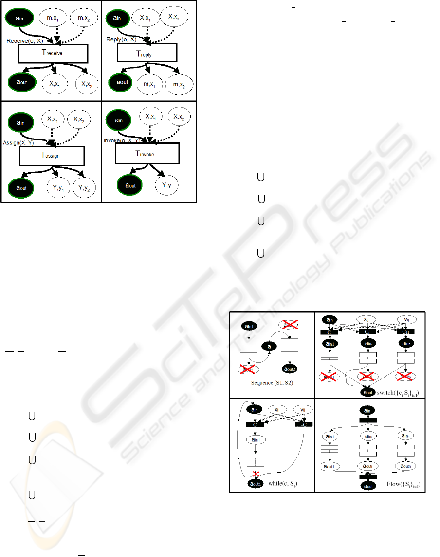
Figure 1: BPEL Petri net models of the basic activities.
• T = T
1
∪ T
2
• C = (C
1
∪ C
2
∪ {(t
i
,a)}
t
i
∈
•
a
out
1
∪ {(a,t
j
)}
t
j
∈a
in
2
•
) \
({(t
i
,a
out
1
)}
t
i
∈
•
a
out
1
∪ {(a
in
2
,t
j
)}
t
j
∈a
in
2
•
)
• R = R
1
∪ R
2
Notice that we introduced an inside activation place a
from T
1
to T
2
.
Conditional operator: the switch operator
switch({(c
i
(
X
i
,V
i
),S
i
)}
i∈I
) represents an alternative
execution of the activities S
i
under the conditions
c
i
(
X
i
,V) where X
i
is the vector of the free variables
x
ij
of the condition and
V
i
is the vector of values v
ij
.
Let N
i
= ha
in
i
,a
out
i
,P
i
,T
i
,C
i
,R
i
i be the BPEL Petri net
model of the activity S
i
. The BPEL Petri net model of
the resulting activity is N = ha
in
,a
out
,P,T,C,Ri with:
• P =
i∈I
(P
i
∪ {a
in
i
} ∪ {x
ij
}
j
∪ {v
ij
}
j
)
• T =
i∈I
(T
i
∪ {t
c
i
})
• C =
i∈I
(C
i
∪ {(a
in
,t
c
i
),(t
c
i
,a
in
i
)} ∪
{(t
ij
,a
out
)}
t
ij
∈
•
a
out
i
) \ {(t
ij
,a
out
i
)}
t
ij
∈
•
a
out
i
• R =
i∈I
(R
i
∪ {(x
ij
,t
c
i
)}
j
∪ {(v
ij
,t
c
i
)}
j
)
Iterative operator: the while operator
while(c(X,V),S
1
) represents an activity that it-
erates the activity S
1
execution until the breaking off
of the conditions c(X) (where X is a vector of the
free variables x
i
and
V is a vector of values v
i
). Let
N
1
= ha
in
1
,a
out
1
,P
1
,T
1
,C
1
,R
1
i be the BPEL Petri net
model of the activity S
1
. The BPEL Petri net model
of the while activity is N = ha
in
,a
out
1
,P,T,C,Ri with:
• P = P
1
∪ {a
in
1
} ∪ {x
i
}
i
∪ {v
i
}
i
• T = T
1
∪ {t
c
,t
c
}
• C = (C
1
∪ {(a
in
,t
c
),(a
in
,t
c
),(t
c
,a
in
1
),(t
c
,a
out
1
)} ∪
{(t
j
,a
in
)}
t
j
∈
•
a
out
1
) \ {(t
j
,a
out
1
)}
t
j
∈
•
a
out
1
• R = R
1
∪ {(x
i
,t
c
),(v
i
,t
c
),(x
i
,t
c
),(v
i
,t
c
)}
i
Notice that we introduced t
c
to represent the transition
if condition c is true and t
c
to represent the transition
if condition c is false.
Parallel operator: the flow operator
flow({S
i
}
i∈I
) executes the activities S
i
in paral-
lel. It terminates when all the activities are finished
(fork-join). Let N
i
= ha
in
i
,a
out
i
,P
i
,T
i
,C
i
,R
i
i be
the BPEL Petri net model of the activity S
i
. The
BPEL Petri net model of the parallel activity is
N = ha
in
,a
out
,P,T,C,Ri with:
• P =
i∈I
(P
i
∪ {a
in
i
,a
out
i
})
• T =
i∈I
T
i
∪ {t
in
,t
out
}
• C =
i∈I
C
i
∪ {(a
in
,t
in
),(t
out
,a
out
} ∪ {(t
in
,a
in
i
)}
i∈I
∪
{(a
out
i
,t
out
)}
i∈I
• R =
i∈I
R
i
Notice that we introduced t
in
and t
out
to represent the
initial and final transitions of the parallel activity.
See the figure 2 for graphical illustration.
Figure 2: BPEL Petri net models of the control operators.
4 ENRICHING BPEL PETRI NET
MODEL FOR DATA
DEPENDENCY
The semantics of the Petri net model and its marking
express the operational dependency between the tran-
MODELING BPEL WEB SERVICES FOR DIAGNOSIS: TOWARDS SELF-HEALING WEB SERVICES
301

sitions executions. But, in addition to this operational
dependency, we want to capture the nature of the de-
pendency between data. For all that, the idea is to
enrich each transition of the BPEL Petri net with a set
of dependency relations (FW, SRC or EL) between
its input and output places. This explicit data causal-
ity together with the Petri net causality properties pro-
vide a rich model to analyze the data dependency in
the BPEL process definition. If P
1
and P
2
are two sets
and F is a set of relations labels between elements of
P
1
and elements of P
2
we will denote by [P
1
→ P
2
]
F
the set of all possible mappings f from P
1
to P
2
such
that ∀p ∈ P
1
, f : p → f(p) ∈ F.
Def 8 The extended BPEL Petri net of the net N =
ha
in
,a
out
,P,T,C,Ri is a tuple EN = hN,Di with
• D : T → 2
[P→P]
{FW,SRC,EL}
such that ∀t ∈ T,D(t) ⊆
[
◦
t ∪
•
t → t
•
]
{FW,SRC,EL}
D is a function that associates to each transition of
the net a set of FW, SRC and EL functions between
the input and output places of the transition.
In the following, we reconsider the BPEL Petri net
model of each BPEL activity and extend it by defining
its D function.
Receive: receive(o,X) receives an input message
and forwards the value contained directly to the vari-
able X, so:
D(t
receive
) = {FW((m,x
i
),(X, x
i
)),FW(a
in
,a
out
)}.
Reply: reply(o,X) just forwards the value of
variable X to the output message, so: D(t
reply
) =
{FW((X,x
i
),(m, x
i
)),FW(a
in
,a
out
)}. Assign: assign(X,Y)
forwards the data of the source variable X to the
target variable Y and assign(v,Y) gives the value
v to the variable Y. In the case of assigning a
variable to a variable, the assign activity only for-
wards the variable value and the activation status
from input to output. And in the case of as-
signing a value to a variable, this (variable,value)
pair is considered as created by the service.
So: D(t
assign
)=

assign(X,Y): {FW(X,Y),FW(a
in
,a
out
)},
assign(v,Y): {SRC(Y), FW(a
in
,a
out
)}.
Invoke: invoke(o,X,Y) is used to call a partner’s op-
eration o. o is known by its intput-output dependency
model a = (X
a
,Y
a
,F
a
). All that we have to do is to ex-
tend the invoke transition by this model, by replacing
in F
a
each x
i
by (X, x
i
) and each y
i
by (Y,y
i
):
D(t
invoke
) = F
a
[x
i
/(X, x
i
),y
i
/(Y, y
i
)] ∪
{FW(a
in
,a
out
)}.
The extended nets of the structured activities are
obtained by composing the extended nets of the activ-
ities in parameters.
Sequence operator: sequence(S
1
,S
2
) does no
add new transition, and it only unifies the input acti-
vation of S
2
with the output activation of S
1
by a new
place labeled a. The data dependency relation does
not change but we relabel the two unified places by a:
D = D
1
[a
out
1
/a] ∪ D
2
[a
in
2
/a].
Conditional operator: the BPEL Petri net model
of switch({(c
i
(
X
i
,V
i
),S
i
)}
i∈I
) has been obtained by
adding a transition t
ci
for each condition, an input ac-
tivation place for the resulting choice, a place for each
variable (or value) involved in each condition c
i
, and
by unifying the output activations of all the activities
S
i
. The switch operator is activated when the input ac-
tivation is transmitted to the activity S
i
whose condi-
tion is evaluated to be true. So it exists an elaboration
relation between the variables and values (x
ij
and v
ij
),
which are used for the c
i
condition evaluation, and the
input activation of S
i
. Each condition transition is thus
extended by an elaboration relation between its input
places (input activation, variables and values) and its
output place:
D =
i∈I
(D
i
[a
out
i
/a
out
] ∪ D(t
ci
))
with D(t
ci
) = {EL({a
in
,x
ij
,v
ij
},a
in
i
)}.
Iterative operator: the BPEL Petri net model of
while(c(
X,V),S
1
) has been obtained by adding two
transitions t
c
and t
c
for the iteration condition c and
its complementary, an input activation place for the
resulting choice between them, and a place for each
variable (or value) involved in the condition. As
for the switch operator, the activation transmission
through one or the other transition is elaborated from
the variables x
i
and values v
i
used in the condition:
D = D
1
[a
out
1
/a
in
] ∪ D(t
c
) ∪ D(t
c
),
with D(t
c
) = {EL({a
in
,x
i
,v
i
},a
in
1
)}
and D(t
c
) = {EL({a
in
,x
i
,v
i
},a
out
1
)}.
Parallel operator: flow({S
i
}
i∈I
) transmits the
activation to each of the activities S
i
. Its BPEL Petri
net model contains two additional transitions: one
that forwards the parallel activation to each activity
and the other that gathers the terminations of each ac-
tivity for ending the parallel activation. So:
D =
i∈I
(D
i
∪ {FW(a
in
,a
in
i
)} ∪ {FW(a
out
i
,a
out
)})
With the enriched BPEL Petri nets defined in this
section, we can capture the data dependency of the
BPEL service operations. But for constructing the di-
agnosis models for BPEL services, we need to define
the propagation rules to aggregate the BPEL service
operations together.
5 PROPAGATING DATA
DEPENDENCIES
As said above, a BPEL process is a partial order ex-
ecution schema on basic activities. As our aim is to
WEBIST 2007 - International Conference on Web Information Systems and Technologies
302

aggregate the BPEL activities models from the basic
ones that compose its code, we are led to compose ex-
tended BPEL Petri nets and thus to define how input-
output dependency relations are aggregated according
to the ”sequential”, ”alternative”, or hierarchical (re-
lated to the XML description) composition.
Let a = h{x},{y},F
a
i and b = h{z},{t},F
b
i
(where x,y,z and t are four data parameters) be the
dependency models of two given activities.
We would like to deduce the dependency model of
the composed activity from:
1. the values of F
a
and F
b
,
2. the unification between parameters,
3. and the execution order model of a and b.
So, we have to axiomatize how dependency relations
f ∈ F
a
and g ∈ F
b
are composed, according to proper-
ties such as ”transitivity” and ”maximality”.
Sequential aggregation rules (f,g): we suppose
here a sequential composition a,b of a and b and
we consider the transitivity axioms. In table 1, we
give the sequential propagation of the three relations
FW,SRC, EL.
Table 1: Sequential aggregation rules.
FW(x, y) FW(z,t)\z = y ≡ FW(x,t)
EL(x,y) EL(z,t)\z = y ≡ EL(x,t)
FW(x, y) EL(z,t)\z = y ≡ EL(x,t)
EL(x,y) FW(z,t)\z = y ≡ EL(x,t)
SRC(y) FW(z,t)\z = y ≡ SRC(t)
SRC(y) EL(z,t)\z = y ≡ SRC(t)
Alternative aggregation rules (f ⊕ g): we sup-
pose here an alternative composition of the depen-
dency models in case of a guarded choice execution.
If c = h{z}, {t},F
c
i is a third activity dependency
model, we consider the activity model d = b⊕c where
either b or c is executed (e.g. following in sequence
the execution of a). The table 2 shows the alternative
composition rules of the three relations FW, SRC,EL
used to express the relation between z and t in the re-
sulted activity d.
Table 2: Alternative aggregation rules.
FW
b
(z,t) ⊕ FW
c
(z,t) ≡ FW
d
(z,t)
EL
b
(z,t) ⊕ FW
c
(z,t) ≡ EL
d
(z,t)
FW
b
(z,t) ⊕ EL
c
(z,t) ≡ EL
d
(z,t)
EL
b
(z,t) ⊕ EL
c
(z,t) ≡ EL
d
(z,t)
SRC
b
(t) ⊕ SRC
c
(t) ≡ SRC
d
(t)
SRC
b
(t) ⊕ FW
c
(z,t) ≡ EL
d
(z,t)
SRC
b
(t) ⊕ EL
c
(z,t) ≡ EL
d
(z,t)
FW
b
(z,t) ⊕ SRC
c
(t) ≡ EL
d
(z,t)
EL
b
(z,t) ⊕ SRC
c
(t) ≡ EL
d
(z,t)
Hierarchical propagation rules through data
structures: the input and output parameters are XML
messages and we need, for diagnosis purpose, to ob-
tain the finest description of the BPEL operations and
thus propagation rules at the level of the messages
substructures. We introduce thus the following de-
composition axioms (a message type being a tree of
labels, for any node label l we denote by X path(l)
the set of all the paths of the subtree of root l):
• FW(l
1
,l
2
) ≡ ∧FW(l
i
,l
j
) with l
i
∈ X path(l
1
), l
j
∈
X path(l
2
) and l
i
≈ l
j
, which means that a forward
relation between two data structures gives rise to
forward relations between all the equivalent (same
type) substructures.
• SRC(l) ≡ ∧SRC(l
j
) with l
j
∈ Xpath(l), which
means that each time a data structure is created,
all its substructures are also created.
• EL(l
1
,l
2
) ≡ ∧EL(l
1
,l
j
) with l
j
∈ X path(l
2
),
which means that if a data structure is elaborated
from another structure, each of its substructures is
also elaborated from this structure.
6 IMPLEMENTING THE BPEL
DIAGNOSIS MODEL
In section 3 and 4, we presented a Petri net modeling
of a BPEL operation and in section 5, we proposed
data dependencies aggregation rules. We can now de-
fine an algorithm that builds the diagnosis model of a
BPEL operation from its extended Petri net. The idea
of the algorithm is based on the following steps:
• Generate all the traces of the Petri net based on an
initial marking and a valid final marking.
• Apply the sequential aggregation rules to each
trace.
• Apply the alternative aggregation rules to the ob-
tained set of aggregated traces.
• Apply the hierarchical propagation rules to data in
order to optimize the operation description.
Let o[m
1
,m
2
] be a BPEL operation mod-
eled by the extended BPEL Petri net N =
ha
in
,a
out
,P,T,C,R,Di. Let M
in
= {a
in
,(m
1
,x
i
),v
j
}
and M = {a
out
,(m
1
,x
i
),v
j
} be the initial and final
markings of N. The set of transitions sequences
FS
M
(S), where S is the net system hN,M
in
i, repre-
sents all the execution paths of N from M
in
to M.
Note that, according to the translating rules, the Petri
net of the BPEL code is finite, but its execution can
be infinite. But such infinite execution can be ex-
pressed using a regular expression. In fact, in our
MODELING BPEL WEB SERVICES FOR DIAGNOSIS: TOWARDS SELF-HEALING WEB SERVICES
303

case, due to the properties of aggregation rules, each
infinite sequence is equivalent to a finite set of fi-
nite sequences. More precisely, taking into account
that any data dependency relation F ∈ {FW, SRC,EL}
verifies F
2
≡ F, we have the equivalences:
F
∗
≡ {ε,F} (ε is the empty sequence) and F
+
≡ {F}.
The diagnosis model of o, R ⊆ [
•
t
receive
∪
◦
t
receive
→
i
t
•
reply
i
]
{FW,SRC,EL}
, is thus given by the algorithm:
Alg 1 Input S: BPEL net system of o, M: final
marking. Output R: set of dependency relations
RF: list of sets of dependency relations
RF =
/
0
for each σ
i
= (t
i1
,t
i2
,...,t
ik
i
) ∈ FS
M
(S) do
R = D(t
i1
);
for j=2 to k
i
do
R = ◦
Agg
(R,D(t
ij
))
endfor;
RF = RF ∪ {R};
endfor;
while (|RF| > 1) do
RF[1] = ⊕
Agg
(RF[1],RF[2]);
remove(RF,RF[2]);
endwhile;
R = RF[1];
7 CONCLUSION
In this paper, following model-based diagnosis ap-
proach, we used Petri nets to construct the diagno-
sis model of a BPEL service. By analyzing its BPEL
code, we decomposed the BPEL process into basic
operations (receive, reply, assign, and invoke) and op-
erators (sequence, switch, while, flow). Each generic
basic operation was then modeled by an extended
BPEL Petri net (normal Petri net enriched by acti-
vation places and reading arcs and extended by data
dependency relations attached to each transition) and
each operator by an extended BPEL Petri net con-
structor, leading to an automatic extended BPEL Petri
net modeling of the process. Finally, we gave the
propagation rules for data dependencies correspond-
ing to several composition modes (sequential, alter-
native, hierarchical through data structures) and the
algorithm for calculating the diagnosis model of a
BPEL service. Such a model can now be used as in-
put to model-based diagnosis algorithms, such as the
one proposed by (Ardissono et al., 2005a).
Further work will be carried out along two steps.
First, achieving decentralized model-based diag-
nosis for composite Web services. All our current
work is in a centralized environment, but in real-
ity, decentralization and distribution are the trends
of software application. Centralized diagnosis is not
adequate for decentralized composite Web services.
Some progress was done in this direction by (Ardis-
sono et al., 2005a), but limited to orchestrated Web
services with a diagnosis supervisor.
Second, realizing auto-repairable and auto-
reconfigurable Web services. For that, we need to
define first the repair and reconfiguration rules for ba-
sic Web service activities (operations or operators),
and then the actions planner and scheduler for the re-
pair and reconfiguration supervisor of the Web ser-
vices (centralized or decentralized).
REFERENCES
Andrews, T., Curbera, F., Dholakia, H., Goland, Y., Klein,
J., Leymann, F., Liu, K., Roller, D., Thatte, S.,
Trickovic, I., and Weerawarana, S. (2003). Busi-
ness process execution language for web services,
version 1.1. BEA Systems, IBM Corp., Microsoft
Corp., SAP AG, Siebel Systems. http://www-
128.ibm.com/developerworks/library/specification/ws-
bpel.
Ardissono, L., Console, L., Goy, A., Petrone, G., Picardi,
C., Segnan, M., and Dupr
´
e, D. T. (2005a). Coop-
ertive model-based diagnosis of web services. Proc. of
IFIP/IEEE Int. Workshop on Self-Managed Systems
Services (SELFMAN 2005), Nice, France.
Ardissono, L., Console, L., Goy, A., Petrone, G., Picardi,
C., Segnan, M., and Dupr
´
e, D. T. (2005b). Enhanc-
ing web services with diagnostic capabilities. Proc. of
European Conference on Web Services (ECOWS-05),
pp. 182-191, Vaxjo, Sweden, IEEE.
Booth, D., Haas, H., McCabe, F., Newcomer, E., Cham-
pion, M., Ferris, C., and Orchard, D. (2004). Web
services architecture, technical report, w3c. Technical
report. http://www.w3.org/TR/ws-arch/.
Hamadi, R. and Benatallah, B. (2003). A petri net-
based model for web service composition. Proc. of
the 14th Australasian database conference, Adelaide,
Australia, ACM.
Hinz, S., Schmidt, H., and Stahl, C. (2005). Trasforminf
bpel to petri nets. Proc. of the 3rd Int. Conference on
Business Process Management (BPM 2005), Nancy,
France, LNCS 3649, pages 220-235.
Rosario, S., Benviniste, A., and S. Haar, C. J. (2006).
Net systems semantics of web services orchestrations
modeled in orc. Research report, IRISA, 1780.
Weerawarana, S. and Curbera, F. (2002). Busi-
ness process with bpel4ws: Understanding
bpel4ws, part 1. Technical report. http://www-
128.ibm.com/developerworks/webservices/library/ws-
bpelcol1/.
WEBIST 2007 - International Conference on Web Information Systems and Technologies
304