
Multinomial Mixture Modelling
for Bilingual Text Classification
Jorge Civera and Alfons Juan
Departament de Sistemes Inform
`
atics i Computaci
´
o
Universitat Polit
`
ecnica de Val
`
encia
46022 Val
`
encia, Spain
Abstract. Mixture modelling of class-conditional densities is a standard pat-
tern classification technique. In text classification, the use of class-conditional
multinomial mixtures can be seen as a generalisation of the Naive Bayes text clas-
sifier relaxing its (class-conditional feature) independence assumption. In this pa-
per, we describe and compare several extensions of the class-conditional multino-
mial mixture-based text classifier for bilingual texts.
1 Introduction
Mixture modelling is a popular approach for density estimation in supervised and un-
supervised pattern classification [1]. On the one hand, mixtures are flexible enough for
finding an appropriate tradeoff between model complexity and the amount of training
data available. Usually, model complexity is controlled by varying the number of mix-
ture components while keeping the same (often simple) parametric form for all compo-
nents. On the other hand, maximum likelihood estimation of mixture parameters can be
reliably accomplished by the well-known Expectation-Maximisation (EM) algorithm.
Although most research on mixture models has concentrated on mixtures for con-
tinuous data, there are many pattern classification tasks for which discrete mixtures are
better suited. This is the case of text classification (categorisation) [2]. In this case, the
use of class-conditional discrete mixtures can be seen as a generalisation of the well-
known Naive Bayes text classifier [3, 4]. In [5], the binary instantiation of the Naive
Bayes classifier is generalised using class-conditional Bernoulli mixtures. Similarly,
in [6,7], its multinomial instantiation is generalised with multinomial mixtures. Both
generalisations seek to relax the Naive Bayes (class-conditional feature) independence
assumption made when using a single Bernoulli or multinomial distribution per class.
This unrealistic assumption of the Naive Bayes classifier is one of the main reasons ex-
plaining its comparatively poor results in contrast to other techniques such as boosting-
based classifier committees, support vector machines, example-based methods and re-
gression methods [2]. In fact, the performance of the Naive Bayes classifier is signifi-
cantly improved by using the generalisations mentioned above [5–7]. Moreover, there
are other recent generalisations (and corrections) that also overcome the weaknesses of
the Naive Bayes classifier and achieve very competitive results [8–12].
In this paper, we describe and compare several (minor) extensions of the (class-
conditional) multinomial mixture-based text classifier for the case in which text data
Civera J. and Juan A. (2006).
Multinomial Mixture Modelling for Bilingual Text Classification.
In 6th International Workshop on Pattern Recognition in Information Systems, pages 93-103
DOI: 10.5220/0002471900930103
Copyright
c
SciTePress

is available in two languages. Our interest in this task of bilingual text classification
comes from its potential use in statistical machine translation. In this application area,
the problem of learning a complex, global statistical transducer from heterogeneous
bilingual sentence pairs can be greatly simplified by first classifying sentence pairs
into homogeneous classes and then learning simpler, class-specific transducers [13].
Clearly, this is only a marginal application of bilingual text classification. More gen-
erally, the proliferation of multilingual documentation in our Information Society will
surely attract many research efforts in multilingual text classification. Obviously, most
conventional, monolingual text classifiers can be also extended in order to fully exploit
the intrinsic redundancy of multilingual texts.
The following section describes the different basic models we consider for multino-
mial mixture modelling of bilingual texts. In section 3, we briefly discuss how to plug
these basic models in the Bayes decision rule for bilingual classification. Section 4
poses the maximum likelihood estimation of these models using the EM algorithm. Fi-
nally, section 5 will be devoted to experimental results and section 6 will discuss some
conclusions and future work.
2 Multinomial Mixture Modelling
A finite mixture model is a probability (density) function of the form:
p(x) =
I
X
i=1
α
i
p(x | i) (1)
where I is the number of mixture components and, for each component i, α
i
∈ [0, 1]
is its prior or coefficient and p(x | i) is its component-conditional probability (density)
function. It can be seen as a generative model that first selects the ith component with
probability α
i
and then generates x in accordance with p(x | i).
The choice of a particular functional form for the components depends on the type
of data at hand and the way it is represented. In the case of the bag-of-words text repre-
sentation, the order in which words occur in a given sentence (or document) is ignored;
the only information retained is a vector of word counts x = (x
1
, . . . , x
D
), where x
d
is the number of occurrences of word d in the sentence, and D is the size of the vo-
cabulary (d = 1, . . . , D). In this case, a convenient choice is to model each component
i as a D-dimensional multinomial probability function governed by its own vector of
parameters or prototype p
i
= (p
i1
, . . . , p
iD
) ∈ [0, 1]
D
,
p(x | i) =
x
+
!
Q
D
d=1
x
d
!
D
Y
d=1
p
x
d
id
(2)
where x
+
=
P
d
x
d
is the sentence length. Equation (1) in this particular case is called
multinomial mixture. Note that the first factor in (2) is a multinomial coefficient giving
the number of different sentences of length x
+
that are equivalent in the sense of having
identical vector of word counts x. Also note that p
id
is the ith component-conditional
probability of word d to occur in a sentence and, therefore, the second factor in (2)
94

is the probability that each of these equivalent sentences has to occur. Thus, Eq. (2)
(and Eq. (1)) defines a explicit probability function over all D-dimensional vectors of
word counts with identical x
+
, and an implicit probability function over all sentences
of length x
+
in which equivalent sentences are equally probable.
In this work, we are interested in modelling the distribution of bilingual texts;
i.e. pairs of sentences (or documents) that are mutual translations of each other. Bilin-
gual texts will be formally described using a direct extension of the bag-of-words rep-
resentation of monolingual text. That is, we have pairs of the form (x, y) in which x is
the bag-of-words representation of a sentence in an input (source) language, and y is its
counterpart in an output (target) language. For instance, x and y may be bag-of-words
in Dutch and English, respectively. As above, x is a D-dimensional vector of words
counts. Regarding y, the size of the output vocabulary will be denoted by E, and thus
y is a E-dimensional vector of word counts y ∈ {0, 1, . . . , y
+
}
E
with y
+
=
P
E
e=1
y
e
.
For modelling the probability of a pair (x, y), we will consider five simple models:
1. Monolingual input-language model:
p(x, y) = p(x) (3)
where p(x) is given by (1) and (2).
2. Monolingual output-language model:
p(x, y) = p(y) (4)
where p(y) is a multinomial mixture model for the output bag-of-words,
p(y) =
I
X
i=1
β
i
p(y | i) with p(y | i) =
y
+
!
Q
E
e=1
y
e
!
E
Y
e=1
q
y
e
ie
(5)
where q
ie
is the ith component-conditional probability of word e to occur in an
output sentence.
3. Bilingual bag-of-words model:
p(x, y) = p(z) (6)
where z is a bilingual bag-of-words obtained from the concatenation of the sen-
tences originating (x, y), and p(z) is a monolingual, multinomial mixture model
like the two previous models.
4. Global (Naive Bayes) decomposition model:
p(x, y) = p(x) p(y) (7)
where p(x) and p(y ) are given by the first two monolingual models above.
5. Local (Naive Bayes) decomposition model:
p(x, y) =
I
X
i=1
γ
i
p(x, y | i) with p(x, y | i) = p(x | i) p(y | i) (8)
where p(x | i) is given by (2) and p(y | i) by (5).
95

Note that the first two models ignore one of the languages involved and hence they
do not take advantage of the intrinsic redundancy in the available data. The remaining
manage bilingual data in slightly different ways.
3 Bilingual Text Classification
As with other types of mixtures, multinomial mixtures can be used as class-conditional
models in supervised classification tasks. Let C denote the number of supervised classes.
Assume that, for each supervised class c, we know its prior p
c
and its class-conditional
probability function, which is given by one of the five models discussed in the previous
section. Then, the Bayes decision rule is to assign each pair (x, y) to a class giving
maximum a posteriori probability or, equivalently,
c(x, y) = argmax
c
log p
c
+ log p(x, y | c) (9)
In the case of the monolingual input-language model, this rule becomes:
c(x, y) = argmax
c
log p
c
+ log
I
X
i=1
α
ci
D
Y
d=1
p
x
d
cid
(10)
Similar rules hold for the monolingual output-language model and the bilingual bag-of-
words model. In the case of the global decomposition model, it is
c(x, y) = argmax
c
log p
c
+ log
I
X
i=1
α
ci
D
Y
d=1
p
x
d
cid
+ log
I
X
i=1
β
ci
E
Y
e=1
q
y
e
cie
(11)
while, in the local decomposition model, we have
c(x, y) = argmax
c
log p
c
+ log
I
X
i=1
γ
ci
D
Y
d=1
p
x
d
cid
E
Y
e=1
q
y
e
cie
(12)
4 Maximum Likelihood Estimation
Let (X, Y ) = {(x
1
, y
1
), . . . , (x
N
, y
N
)} be a set of samples available to learn one of
the five mixture models discussed in section 2. This is a statistical parameter estimation
problem since the mixture is a probability function of known functional form, and all
that is unknown is a parameter vector including the priors and component prototypes.
In what follows, we will focus on the local decomposition model; the rest of models
can be estimated in a similar way.
The vector of unknown parameters for the local decomposition model is:
Θ = (γ
1
, . . . , γ
I
; p
1
, . . . , p
I
; q
1
, . . . , q
I
) (13)
We are excluding the number of components from the estimation problem, as it is a cru-
cial parameter to control model complexity and receives special attention in Section 5.
96

Following the maximum likelihood principle, the best parameter values maximise
the log-likelihood function
L(Θ|X, Y ) =
N
X
n=1
log
I
X
i=1
γ
i
p(x
n
|i) p(y
n
|i) (14)
In order to find these optimal values, it is useful to think of each sample pair (x
n
, y
n
)
as an incomplete component-labelled sample, which can be completed by an indica-
tor vector z
n
= (z
n1
, . . . , z
nI
) with 1 in the position corresponding to the component
generating (x
n
, y
n
) and zeros elsewhere. In doing so, a complete version of the log-
likelihood function (14) can be stated as
L
C
(Θ|X, Y,Z) =
N
X
n=1
I
X
i=1
z
ni
log γ
i
+ log p(x
n
|i) + log p(y
n
|i)
(15)
where Z = {z
1
, . . . , z
N
} is the so-called missing data.
The form of the log-likelihood function given in (15) is generally preferred because
it makes available the well-known EM optimisation algorithm (for finite mixtures) [14].
This algorithm proceeds iteratively in two steps. The E(xpectation) step computes the
expected value of the missing data given the incomplete data and the current parameters.
The M(aximisation) step finds the parameter values which maximise (15), on the basis
of the missing data estimated in the E step. In our case, the E step replaces each z
ni
by
the posterior probability of (x
n
, y
n
) being actually generated by the ith component,
z
ni
=
γ
i
p(x
n
| i) p(y
n
| i)
P
I
i
′
=1
γ
i
′
p(x
n
| i
′
) p(y
n
| i
′
)
(16)
for all n = 1, . . . , N and i = 1, . . . , I, while the M step finds the maximum likelihood
estimates for the priors,
γ
i
=
1
N
N
X
n=1
z
ni
(i = 1, . . . , I) (17)
and the component prototypes,
p
i
=
1
P
N
n=1
z
ni
P
D
d=1
x
nd
N
X
n=1
z
ni
x
n
q
i
=
1
P
N
n=1
z
ni
P
E
e=1
y
ne
N
X
n=1
z
ni
y
n
(18)
for all i = 1, . . . , I.
The above estimation problem and algorithm are only valid for a single multino-
mial mixture of the form (8). Nevertheless, it is straightforward to extend them in
order to simultaneously work with several class-conditional mixtures in a supervised
setting. In this setting, training samples come with their corresponding class labels,
{(x
n
, y
n
, c
n
)}
N
n=1
, and the vector of unknown parameters is:
Ψ = (p
1
, . . . , p
C
; Θ
1
, . . . , Θ
C
) (19)
97

where, for each supervised class c, its prior probability is given by p
c
and its class-
conditional probability function is a mixture controlled by a vector of the form (13),
Θ
c
. The log-likelihood of Ψ w.r.t. the labelled data is
L=
N
X
n=1
log p
c
n
I
X
i=1
γ
c
n
i
p(x
n
|i, c
n
)p(y
n
|i, c
n
) (20)
which can be optimised by a simple extension of the EM algorithm given above. More
precisely, the E step computes (16) using Θ
c
n
, while the M step computes the conven-
tional estimates for the class priors and (class-dependent versions of) Eqs. (17) to (18)
for each class separately. This simple extension of the EM algorithm is equivalent to the
usual practice of applying its basic version to each supervised class in turn. However,
we prefer to adopt the extended EM, mainly to have a unified framework for classifier
training in accordance with the log-likelihood criterion (20).
5 Experimental Results
The five different models considered were assessed and compared on two bilingual
text classification datasets (tasks) known as the Traveller dataset and the BAF corpus.
The Traveller dataset comprises Spanish-English sentence pairs drawn from a restricted
semantic domain, while BAF is a parallel French-English corpus collected from a mis-
cellaneous ”institutional” document pool. This section first describes these datasets and
then provides the experimental results obtained.
5.1 Datasets
The Traveller dataset comes from a limited-domain Spanish-English machine transla-
tion application for human-to-human communication situations in the front-desk of a
hotel [15]. It was semi-automatically built from a small “seed” dataset of sentence pairs
collected from traveller-oriented booklets by four persons. Note that each person had to
cater for a (non-disjoint) subset of subdomains, and thus each person can be considered
a different (multimodal) class of Spanish-English sentence pairs. Subdomain overlap-
ping among classes foresees that perfect classification is not possible, although in our
case, low classification error rates will indicate that our mixture model has been able to
capture the multimodal nature of the data. Unfortunately, the subdomain of each pair
was not recorded, and hence we cannot train a subdomain-supervised multinomial mix-
ture in each class to see how it compares to mixtures learnt without such supervision.
The Traveller dataset contains 8, 000 sentence pairs, with 2, 000 pairs per class. The
size of the vocabulary and the number of singletons reflect the relative simplicity of this
corpus. Some statistics are shown in Table 1.
The BAF corpus [16] is a compilation of bilingual ”institutional” French-English
texts ranging from debates of the Canadian parliament (Hansard), court transcripts and
UN reports to scientific, technical and literary documents. This dataset is composed of
11 documents that are organised into 4 natural genres (Institutional, Scientific, Tech-
nical and Literary) trying to be representative of the types of text that are available in
98

multilingual versions. Institutional and Scientific classes comprises documents from the
original pool of 11 documents, which were theme-related, but devoted to heterogeneous
purposes or written by different authors. This fact provides the multimodal nature to the
BAF corpus that can be adequately modelled by mixture models. The BAF corpus was
aligned at the sentence level by human experts and it was initially thought to be used as
a reference corpus to evaluate automatic alignment techniques in machine translation.
Prior to performing the experiments, the BAF corpus was simplified in order to re-
duce the size of the vocabulary and discard spurious sentence pairs. This preprocessing
mainly consisted in three basic actions: downcasing, replacement of those words con-
taining a sequence of numbers by a generic label, and isolation of punctuation marks.
This basic procedure halved the size of the vocabulary and significantly simplified this
corpus. Neither stopword lists, nor stemming techniques were applied since, as shown
in [8], it is unclear whether this further preprocessing may be convenient. As it can be
seen in Table 1, this corpus is more complex than the Traveller dataset.
Table 1. Traveller and BAF corpora statistics.
Traveller BAF
Sp En Fr En
sentence pairs 8000 18509
average length 9 8 28 23
vocabulary size 679 503 20296 15325
singletons 95 106 8084 5281
running words 86K 80K 522K 441K
5.2 Experimental Results
Several experiments were carried out to analyse the behaviour of each individual clas-
sifier in terms of log-likelihood and classification error rate as a function of the number
of mixture components per class (I ∈ {1, 2, 5, 10, 20, 50, 100}). This was done for a
training and test sets resulting from a random dataset partition (1/2-1/2 split for Trav-
eller and 4/5-1/5 for BAF).
Figure 1 shows the evolution of the error rate (left y axis) and log-likelihood (right
y axis), on training and test sets, for an increasing number of mixture components (x
axis). From top to bottom rows we have: the best monolingual classifier (English in
both datasets), the bilingual bag-of-words classifier, and global and local classifiers.
Each plotted point is an average over values obtained from 30 randomised trials.
From the results in Figure 1, we can see that the evolution of the log-likelihood on
the training and test sets is as theoretically expected, for all classifiers in both, Traveller
and BAF. The log-likelihood in training always increases, while the log-likelihood in
test increases up to a moderate number of components (20 − 50 in Traveller and 5 −
10 in BAF). This number of components can be considered as an indication of the
number of “natural” subclasses in the data. About this number of mixture components
99

is also commonly found the lowest classification test error rate, as it occurs in our case.
As the number of components keeps increasing, the well-known overtraining effect
appears, the log-likelihood in test falls and the accuracy degrades. For this reason we
decided to limit the number of mixture components to 100, since additional trials with
an increasing number of mixture components confirmed this performance degradation.
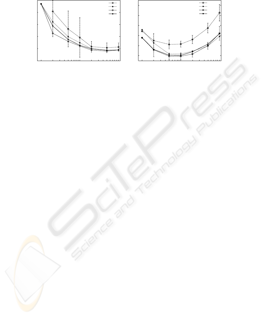
Figure 2 shows competing curves for test error-rate as a function of the number of
mixture components for the English-based, bilingual bag-of-words-based, global and
local classifiers; there are two plots, one for Traveller and the other for BAF. Error bars
representing 95% confidence intervals are plotted for the English-based classifiers in
both plots, and the global classifier in BAF.
From the results for Traveller in Figure 2, we can see that there is no significant
statistical difference in terms of error rate between the best monolingual classifier and
the bilingual classifiers. The reason behind these similar results can be better explained
in the light of the statistics of the Traveller dataset shown in Table 1. The simplicity of
the Traveller dataset, characterised by its small vocabulary size and its large number of
running words, allows for a reliable estimation of model parameters in both languages.
This is reflected in the high accuracy (∼ 95%) of the monolingual classifiers and the
little contribution of a second language to boost the performance of bilingual classifiers.
Nevertheless, bilingual classifiers seem to achieve systematically better results.
In contrast to the results obtained for Traveller, the results for BAF in Figure 2 in-
dicate that bilingual classifiers perform significantly better than monolingual models.
More precisely, if we compare the curves for the English-based classifier and the global
classifier, we can observe that there is no overlapping between their error-rate confi-
dence intervals. Clearly, the complexity and data scarcity problem of the BAF corpus
lead to poorly estimated models, favouring bilingual classifiers that take advantage of
both languages. However, the different bilingual classifiers have similar performance.
Additional experiments using smooth n-gram language models were performed
with the well-known and publicly available SRILM toolkit [17]. A Witten-Bell [18]
smoothed n-gram language model was trained for each supervised class separately and
for both languages independently. These class-dependent language models were used to
define monolingual and bilingual Naive Bayes classifiers. Results are given in Table 2.
From the results in Table 2, we can see that 1-gram language models are similar
to our 1-component mixture models. In fact, both models are equivalent except for the
parameter smoothing. The results obtained with n-gram classifiers with n > 1 are much
better that the results for n = 1 and slightly better than the best results obtained with
general I-component multinomial mixtures. More precisely, the best results achieved
with n-grams are 1.1% in Traveller and 2.6% in BAF, while the best results obtained
with multinomial mixtures are 1.4% in Traveller and 2.9% in BAF.
Table 2. Test-set error rates for monolingual and bilingual naive classifiers based on smooth
n-gram language models in Traveller and BAF.
Traveller 1-gram 2-gram 3-gram
English classifier 4.1 1.9 1.3
Spanish classifier 2.8 1.2 1.2
Bilingual classifier 3.3 1.2 1.1
BAF 1-gram 2-gram 3-gram
English classifier 5.3 3.5 3.6
French classifier 6.7 4.4 4.4
Bilingual classifier 4.1 2.8 2.6
100

0.0
0.5
1.0
1.5
2.0
2.5
3.0
3.5
4.0
1 2 5 10 20 50 100
-50
-45
-40
-35
-30
Error (%) Log-Likelihood
Mixture components
Training
Log-L
Test
Log-L
Test
Error
Training
Error
Traveller dataset
English-based classifier
0
1
2
3
4
5
6
7
8
9
10
100502010521
-190
-180
-170
-160
-150
-140
-130
-120
Error (%) Log-Likelihood
Mixture components
Test
Error
Training
Log-L
Training
Error
Test
Log-L
BAF dataset
English-based classifier
0.0
0.5
1.0
1.5
2.0
2.5
3.0
3.5
4.0
1 2 5 10 20 50 100
-95
-90
-85
-80
-75
-70
Error (%) Log-Likelihood
Mixture components
Training
Log-L
Test
Log-L
Test
Error
Training
Error
Traveller dataset
BBoW-based classifier
0
1
2
3
4
5
6
7
8
9
10
1 2 5 10 20 50 100
-380
-370
-360
-350
-340
-330
-320
-310
Error (%) Log-Likelihood
Mixture components
Test
Error
Training
Log-L
Training
Error
Test
Log-L
BAF dataset
BBoW-based classifier
0.0
0.5
1.0
1.5
2.0
2.5
3.0
3.5
4.0
1 2 5 10 20 50 100
-95
-85
-75
-65
-55
Error (%) Log-Likelihood
Mixture components
Test
Error
Training
Log-L
Training
Error
Test
Log-L
Traveller dataset
Global classifier
0
1
2
3
4
5
6
7
8
9
10
1 2 5 10 20 50 100
-380
-360
-340
-320
-300
-280
Error (%) Log-Likelihood
Mixture components
Test
Error
Training
Log-L
Training
Error
Test
Log-L
BAF dataset
Global classifier
0.0
0.5
1.0
1.5
2.0
2.5
3.0
3.5
4.0
1 2 5 10 20 50 100
-95
-85
-75
-65
-55
Error (%) Log-Likelihood
Mixture components
Test
Error
Training
Log-L
Training
Error
Test
Log-L
Traveller dataset
Local classifier
0
1
2
3
4
5
6
7
8
9
10
1 2 5 10 20 50 100
-380
-360
-340
-320
-300
-280
Error (%) Log-Likelihood
Mixture components
Test
Error
Training
Log-L
Training
Error
Test
Log-L
BAF dataset
Local classifier
Fig.1. Error rate and log-likelihood curves in training and test sets as a function of the number
of mixture components, in Traveller (left column) and BAF (right column) for the four classifiers
considered. Classifiers: the best monolingual, the bilingual bag-of-words (BBoW), the global and
the local classifier.
101
1.0
1.5
2.0
2.5
3.0
3.5
1 2 5 10 20 50 100
Error (%)
Mixture components
Traveller dataset
English-based classifier
Bilingual-BoW-based classifier
Global classifier
Local classifier
3.0
4.0
5.0
6.0
7.0
8.0
1 2 5 10 20 50 100
Error (%)
Mixture components
BAF dataset
English-based classifier
Bilingual-BoW-based classifier
Global classifier
Local classifier
Fig.2. Test-set error rate curves as a function of the number of mixture components, for each
classifier in Traveller (left) and BAF (right).
6 Conclusions and Future Work
We have presented three different extensions of the multinomial mixture-based text
classification model for bilingual text: the bilingual bag-of-words model and the global
and local decomposition models. The performance of these extensions was compared
to that of monolingual and smooth n-gram classifiers. Two outstanding conclusions
can be stated from the results presented. First, mixture-based classifiers surpass single-
component classifiers in all cases (monolingual, bilingual bag-of-words, global and
local). In fact, we have taken advantage of the flexibility of the mixture modelisa-
tion over the ”single-component” approach to further improve the error rates achieved.
This mixture modelling superiority is also reflected in the monolingual versions of our
text classifiers and corroborated through smooth n-gram language model experiments
with independent software. Second, bilingual classifiers outperform their monolingual
and smooth 1-gram counterparts, and the excellence of bilingual classifiers is more
clearly shown when the complexity of the dataset does not allow for monolingual well-
estimated models, as in the BAF corpus. Therefore, the contribution of an extra source
of information instantiated as a second language cannot be neglected.
As a future work, smooth n-gram language models for bilingual text classifica-
tion provide an interesting starting point for future research based on more versatile
language models, as mixtures of bilingual n-gram language models. A promising ex-
tension of this work would be the development of mixture of 2-gram language models.
All in all, the bilingual approaches described in this work are relatively simple mod-
els for the statistical distribution of bilingual texts. More sophisticated models, such as
IBM statistical translation models [19], may be better in describing the statistical dis-
tribution of bilingual, correlated texts.
102

References
1. Jain, A.K., et al.: Statistical Pattern Recognition: A Review. IEEE Trans. on PAMI 22 (2000)
4–37
2. Sebastiani, F.: Machine learning in automated text categorisation. ACM Comp. Surveys 34
(2002) 1–47
3. Lewis, D.D.: Naive Bayes at Forty: The Independence Assumption in Information Retrieval.
In: Proc. of ECML’98. (1998) 4–15
4. McCallum, A., Nigam, K.: A Comparison of Event Models for Naive Bayes Text Classifi-
cation. In: AAAI/ICML-98 Workshop on Learning for Text Categorization. (1998) 41–48
5. Juan, A., Vidal, E.: On the use of Bernoulli mixture models for text classification. Pattern
Recognition 35 (2002) 2705–2710
6. Nigam, K., et al.: Text Classification from Labeled and Unlabeled Documents using EM.
Machine Learning 39 (2000) 103–134
7. Novovicov
´
a, J., Mal
´
ık, A.: Application of Multinomial Mixture Model to Text Classification.
In: Proc. of IbPRIA 2003. (2003) 646–653
8. Vilar, D., et al.: Effect of Feature Smoothing Methods in Text Classification Tasks. In: Proc.
of PRIS’04. (2004) 108–117
9. Pavlov, D., et al.: Document Preprocessing For Naive Bayes Classification and Clustering
with Mixture of Multinomials. In: Proc. of KDD’04. (2004) 829–834
10. Peng, F., et al.: Augmenting Naive Bayes classifiers with statistical language models. Infor-
mation Retrieval 7 (2003) 317–345
11. Rennie, J., et al.: Tackling the Poor Assumptions of Naive Bayes Text Classifiers. In: Proc.
of ICML’03. (2003) 616–623
12. Scheffer, T., Wrobel, S.: Text Classification Beyond the Bag-of-Words Representation. In:
Proc. of ICML’02 Workshop on Text Learning. (2002)
13. Cubel, E., et al.: Adapting finite-state translation to the TransType2 project. In: Proc. of
EAMT/CLAW’03, Dublin (Ireland) (2003) 54–60
14. Dempster, A.P., et al.: Maximum likelihood from incomplete data via the EM algorithm
(with discussion). Journal of the Royal Statistical Society B 39 (1977) 1–38
15. Vidal, E., et al.: Example-Based Understanding and Translation Systems. Report ESPRIT
project (2000)
16. Simard, M.: The BAF: A Corpus of English-French Bitext. In: Proc. of LREC’98. (1998)
489–496
17. Stolcke, A.: SRILM – an extensible language modeling toolkit. In: Proc. of ICSLP’02.
Volume 2. (2002) 901–904
18. Witten, I.H., et al.: The zero-frequency problem: Estimating the probabilities of novel events
in adaptive text compression. IEEE Trans. on Information Theory 37 (1991) 1085–1094
19. Brown, P.F., et al.: A Statistical Approach to Machine Translation. Comp. Linguistics 16
(1990) 79–85
103
