IMAGE TRANSMISSION WITH ADAPTIVE POWER AND RATE
ALLOCATION OVER FLAT FADING CHANNELS USING JOINT
SOURCE CHANNEL CODING
Greg H. H
˚
akonsen, Tor A. Ramstad and Anders Gjendemsjø
Department of Electronics and Telecommunications, Norwegian University of Science and Technology
O.S. Bragstads plass 2B, 7491 Trondheim, Norway.
Keywords:
Joint source channel coding, nonlinear mappings, fading channel, image coder.
Abstract:
A joint source channel coder (JSCC) for image transmission over flat fading channels is presented. By letting
the transmitter have information about the channel, and by letting the code-rate vary slightly around a target
code-rate, it is shown how a robust image coder is obtained by using time discrete amplitude continuous
symbols generated through the use of nonlinear dimension changing mappings. Due to their robustness these
mappings are well suited for the changing conditions on a fading channel.
1 INTRODUCTION
For transmission over wireless channels it is impor-
tant to have a robust system as the channel conditions
vary as a function of time. Traditional tandem sys-
tems use a channel code that is designed for a worst
case channel signal-to-noise ratio (CSNR) where it
can guarantee a bit error rate (BER) below a certain
level. A source coder is then matched to the bit rate
for which the channel code is designed. There are
two main problems with this system. One is that this
system breaks down very fast if the true CSNR falls
below the design level. On the other hand, if the true
CSNR is much higher than the design level, this sys-
tem suffers from what is called the leveling-off effect.
As the CSNR rises, the BER decreases, but the perfor-
mance of the system remains constant after a certain
threshold. This is due to the lossy part of the source
coder: the design of the quantizer sets a certain distor-
tion level which yields the target rate of the channel
code.
To increase the average bit rate over a channel, one
strategy is to divide the CSNR range into a set of re-
gions and use different constellations for the different
regions, see e.g. (Holm et al., 2003). This does not,
however, combat the problem that most channel codes
need to group very long bit sequences into blocks to
perform well. So switching fast between these con-
stellations becomes a problem.
Shannon’s separation theorem (Shannon, 1948),
says that a source coder and channel coder can be sep-
arately designed and still obtain an optimal communi-
cation system. To achieve this, the two coders have to
have infinite complexity and infinite delay. When tak-
ing complexity and delay into account, joint source
channel coding (JSCC) is a promising solution. The
idea in JSCC is to optimize the source and channel
codes together, and in that manner make the source
information better adapted to the channel. Work on
JSCC can be split into three main categories, one is
fully digital systems, where the different parts of the
source is given unequal error protection (UEP) on
the channel, see e.g. (Tanabe and Farvardin, 1992).
A second is hybrid digital-analog (HDA) systems,
where some digital information is sent, but an analog
component is sent as refinement, see e.g. (Mittal and
Phamdo, 2002). In this paper the focus is on contin-
uous amplitude systems, where the main information
is sent without any kind of channel code. We use non-
linear Shannon mappings to adapt the transmission of
an image over a flat fading channel without the use of
any quantization or channel codes. This image com-
munication system is partly based on the system pre-
sented for an additive white Gaussian noise (AWGN)
channel in (Coward and Ramstad, 2000).
2 SYSTEM OVERVIEW
The system considered in this paper is a joint source
channel coder for image transmission over flat fading
158
H. Hakonsen G., A. Ramstad T. and Gjendemsjø A. (2006).
IMAGE TRANSMISSION WITH ADAPTIVE POWER AND RATE ALLOCATION OVER FLAT FADING CHANNELS USING JOINT SOURCE CHANNEL
CODING.
In Proceedings of the International Conference on Wireless Information Networks and Systems, pages 158-163
Copyright
c
 SciTePress

Channel
channel
estimator
Perfect
n(k) α(k)
Classification
Preallocation/
mapping
allocation
Adaptive
image
Source
Power
Cont rol
CSI
Transmitter
Analysis
filter bank
Mapping 1
Mapping J
.
.
.
P(k)
Side info
CSI
Receiver
Synthesis
image
Decoded
filter bank
Channel gain
Demapping mismatch
equalizer
Side info
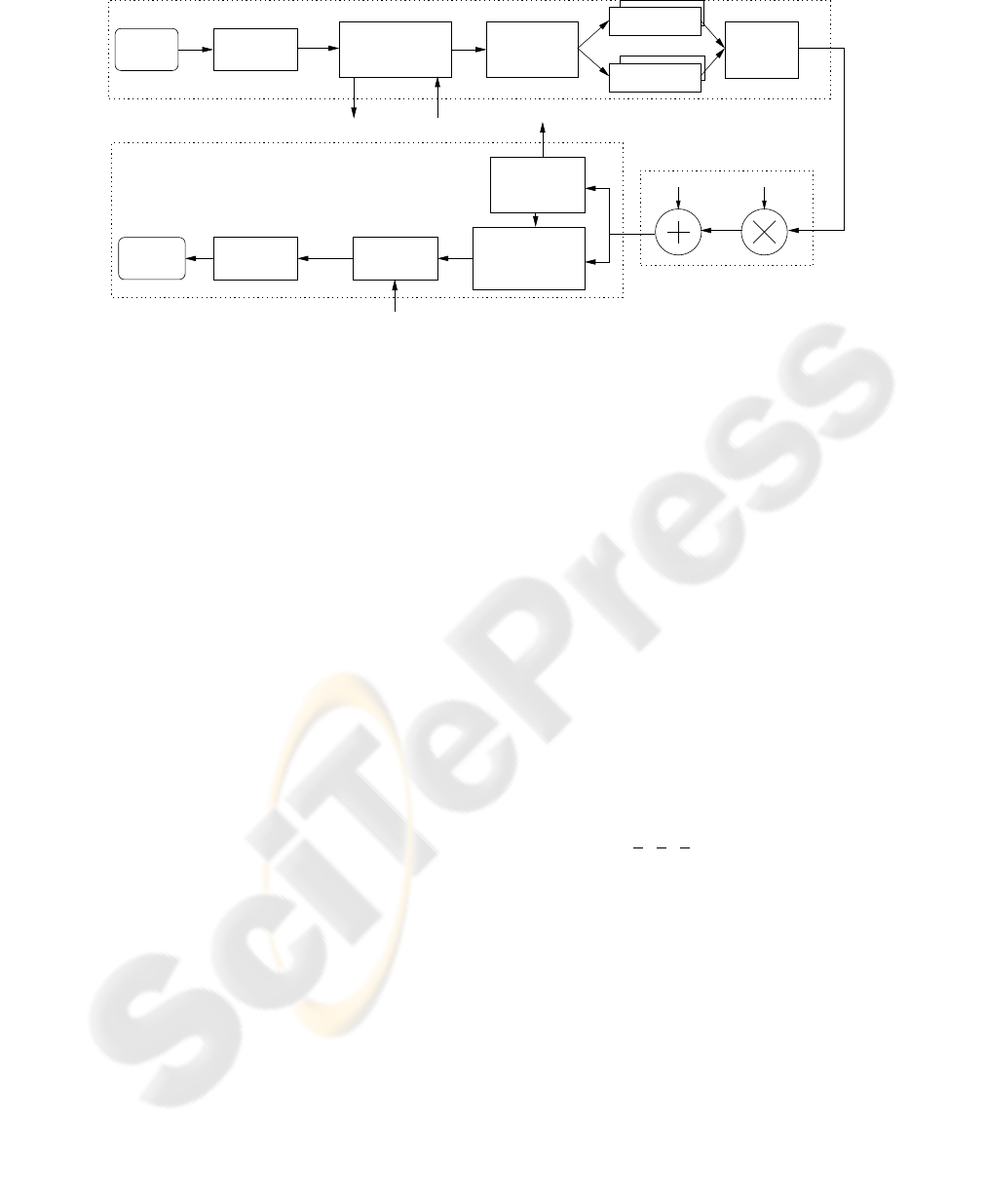
Figure 1: Proposed image transmission system.
channels. The structure of the system is as seen in
Figure 1.
We assume that the return channel from the receiver
to the transmitter has no delay, so that the transmit-
ter has the same information as the receiver about the
channel. To be able to decode the main information,
the receiver needs some side information. The side
information sent from the transmitter is assumed to
be error free. At least at high rates, the size of the side
information will have little impact on the total band-
width. Any further investigation of the size of the side
information is outside the scope of this paper. Trans-
mission and coding are based on the use of nonlin-
ear dimension changing mappings. The properties for
these mappings will not be analyzed here, but can be
found in e.g., (Coward and Ramstad, 2000; Fuldseth
and Ramstad, 1997). The channel samples are trans-
mitted as amplitude continuous, time discrete PAM
symbols. The mappings work by taking g source sam-
ples and represent these samples by b channel sam-
ples, where g and b are integers such that ˆr = b/g.
The resulting ratio ˆr, will from now on be denoted as
the rate of the mapping. A mapping of ˆr = 2 repre-
sents each source sample as 2 channel samples, thus
adding redundancy to protect that sample.
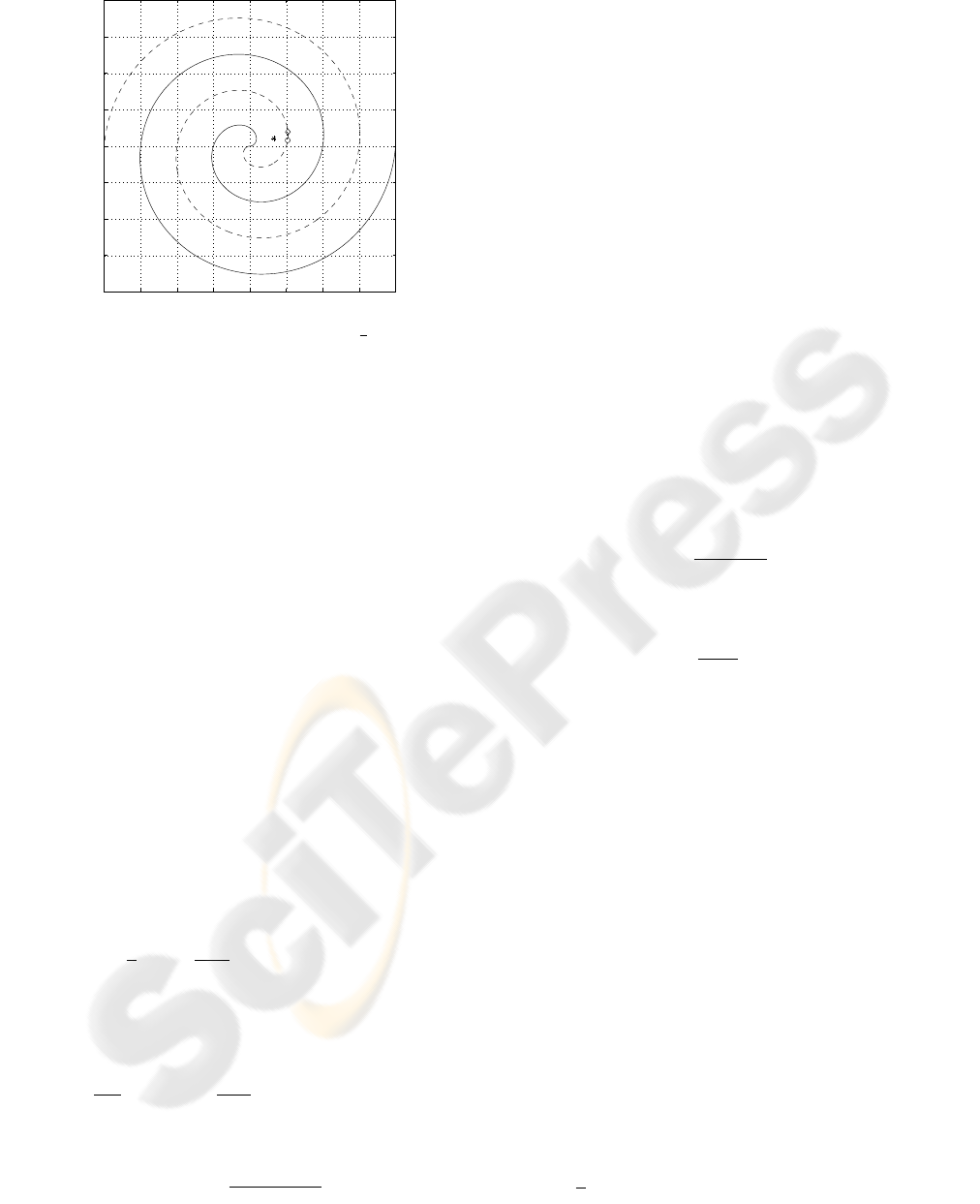
A mapping of ˆr = 1/2 is shown in Figure 2. Com-
pression is achieved by representing two source sam-
ples by one channel sample. A 2D vector composed
of two source samples is represented by (*). This
point is then mapped to the closest point on the spiral,
represented by (o). This point will then be transmit-
ted as a continuous amplitude PAM symbol. Points on
the dotted line can be represented by negative channel
symbols, while points on the solid line can be repre-
sented by positive channel symbols. Channel noise
will move this point so that the received point will
have a different value, represented by (♦). The total
distortion in the reconstructed sample will be due to
the approximation and channel noise.
Figure 2 can also be used to explain a mapping of
ˆr = 2. Letting the spiral represent the source space,
a source sample, represented by (♦), can take any
value along the spiral. By representing this sample
as a 2D vector, the value of each coordinate can be
transmitted as a continuous amplitude PAM symbol.
After noise is added, the resulting 2D vector has been
moved in the noise-space, represented by (*). The re-
ceiver knows that the original point has to be on the
spiral, and maps it into the closest point along the spi-
ral, represented by (o).
Designing good mappings for large dimension
changes is increasingly more difficult as the dimen-
sionality goes up, due to the high number of parame-
ters that need to be optimized, similar to vector quan-
tization (Gersho and M. Gray, 1992). Due to this, the
mappings we use in this paper have rates
ˆr
j
∈ {0,
1
4
,
1
2
,
2
3
, 1, 2}, j = 0, . . . , 5. (1)
Each mapping can be optimally designed for a set of
given CSNRs, {γ
m
}
M
m=1
. The obtained signal repre-
sentations are robust, so the system improves and de-
grades the performance gracefully around the design
CSNR.
2.1 Source Description
The source in this paper is an image which is decorre-
lated by using a filter bank designed by Balasingham
in (Balasingham, 1998). This filter bank consists of
an 8 × 8 band uniform filter bank, and three different
2×2 band filter banks, used in a tree structure so each
filter is applied to the low-low band of the previous
stage. The filter bank is maximally decimated which

−4 −3 −2 −1 0 1 2 3 4
−4
−3
−2
−1
0
1
2
3
4
Figure 2: Example of mapping with r
j
=
1
2
. 2D input
vector marked by (*) is mapped to the closest point (o) in
the channel space (the spiral). The channel noise will move
the point along the spiral (♦).
keeps the number of pixels equal before and after fil-
tering. Images have non-zero means, which implies
a non-zero mean in the resulting low-low band, so to
reduce the power of the image, the mean is subtracted
from this band and sent as side information.
To cope with the local statistical differences within
each band, the subband filtered image is split into N
blocks. By using small blocks, the local statistics are
captured better, but then the number of blocks will
be larger, resulting in larger side information. To
be able to decode the transmitted signal the receiver
needs knowledge about the variances of all the source
blocks. This information is sent as side information.
Taking practical considerations into account, we have
found 8 ×8 subband pixels to be a suitable block size.
The variance σ
2
X
n
of each block is estimated using the
RMS value.
We assume that the transform coefficients within a
block can be modeled by a Gaussian pdf (Lervik and
Ramstad, 1996). For a given distortion µ, the block
variance can then be used to find the rate (bits/source
sample), for each sub-source(block) from the follow-
ing expression (Berger, 1971),
R
n
=
1
2
log
2

σ
2
X
n
σ
2
D
n

bits/source sample, (2)
where σ
2
D
n
= min(µ, σ
2
X
n
).
Assuming that all the N blocks are independent,
the total average rate is given by
R =
1
2N
N−1
X
n=0
log
2

σ
2
X
n
σ
2
D
n

bits/source sample. (3)
The overall signal-to-noise ratio (SNR) is given by
SNR =
P
N−1
n=0
σ
2
X
n
P
N−1
n=0
σ
2
D
n
. (4)
By using (4), it is possible to find the value of µ that
yields a wanted SNR. This can be the scenario if the
receiver needs a certain quality in the received image.
Another scenario is when there is a time requirement,
i.e. the transmission has be be finished within a cer-
tain time. This will put a rate constraint on (3), and the
corresponding µ for this rate needs to be found. Large
values of µ imply that some of the source blocks are
discarded according to rate distortion theory (Berger,
1971).
2.2 Channel Adaptation
We consider a frequency-flat fading channel where it
is assumed that the received signal y(k) can be written
as
y(k) = α(k)v(k) + n(k), (5)
where α(k) is a stationary channel gain, v(k) is the
sent signal and n(k) is AWGN.
Let
¯
P denote the average transmit power and N
0
/2
be the noise density on the channel of bandwidth B.
The instantaneous CSNR, γ(k), is defined as
γ(k) =
¯
P |α(k)|
2
N
0
B
, (6)
and let the expected value of the CSNR, ¯γ, be
¯γ =
¯
P
N
0
B
. (7)
To avoid an infinite amount of channel state infor-
mation (CSI), the CSNR range is divided into M + 1
regions, similar to e.g. (Holm et al., 2003). In this
paper we choose to let a set of parameters {γ
m
}
M
m=1
represent the different CSNR regions where we trans-
mit, and let the region with worst CSNR represent
outage. These regions will be denoted as channel
states. The representation points γ
m
, are placed inside
each channel region similar to representation points
in scalar quantization. The reason why this system
is optimized for a representation point within a re-
gion instead of the edges which is common in adap-
tive coded modulation (ACM), is that the mappings
used in this system degrades and improves gracefully
in an area around the design CSNR instead of break-
ing down as is the case of conventional digital codes.
So a mismatch between the CSNR for which a map-
ping is coded, and the actual CSNR, does not have so
big impact as it would in traditional systems.
For a channel state γ
m
, the instantaneous channel
capacity is then given by, for m = 1, . . . , M,
C
m
=
1
2
log
2
(1 + γ
m
) bits/channel sample. (8)

2.3 Matching Source to Channel
Since the source is represented by source blocks, and
the channel is divided into discrete channel states, it
is interesting to look at the instantaneous rate, given
by
r
n,m
=
log
2

σ
2
X
n
σ
2
D
n

log
2
(1 + γ
m
)
channel/source samples. (9)
For a given channel state γ
m
, (9) gives the rate-
change needed to be able to transmit a source block
with variance σ
2
X
n
and distortion µ. Using a contin-
uous set of dimensional changing mappings is, how-
ever, highly impractical, so in practice r
n,m
has to be
approximated to the closest match in (1). And since
the mappings are not ideal, the actual performance of
each mapping has to be considered.
To set up a reasonable strategy for source-channel
adaptation, the different source blocks are preallo-
cated to the different channel states so that the block
with largest variance is matched with the best chan-
nel state. The preallocation is done using the long
term statistics of the channel. For a single transmis-
sion the channel does not behave exactly according to
the statistics. So if, during transmission, there are no
more blocks preallocated to a given state, blocks from
a better channel state are transmitted, but then a new
mapping has to be used calculated from (9). In this
way the system can adapt to the varying conditions of
the channel.
2.4 Finding the Representation
Points
Since the source blocks are preallocated to different
channel states, it is natural to include them in the cal-
culation of channel representation points γ
m
. Find-
ing the best representation points γ
m
will also include
finding the best thresholds ˆγ
m
that defines the differ-
ent channel regions R
m
= {γ : ˆγ
m
< γ ≤ ˆγ
m+1
}.
Since the rate-change needed is given by the ratio
between the source rate and instantaneous channel ca-
pacity, (9), it is natural to include this into the op-
timization problem. By looking at the total average
rate-change needed in a given channel state m
r
avg
m
(γ
m
) =
1
|I
m
|
P
n∈I
m
log
2
(
σ
2
X
n
σ
2
D
n
)
log
2
(1 + γ
m
)
, (10)
where I
m
is the set of source blocks allocated to the
m’th channel state, we can find the mean squared
error (MSE) denoted, ǫ, for all the M transmission
channel states and all source blocks by
ǫ =
M
X
m=1
Z
R
m

r
avg
m
(γ) − r
avg
m
(γ
m
)

2
p
γ
(γ)dγ.
(11)
Minimization of ǫ with respect to R
m
and γ
m
has to
be done through an iteration process, since the num-
ber of blocks in each channel state varies.
2.5 Optimization of Power
Distribution
The mapping rate, ˆr
n
, for each block, does not match
the needed rate r
n,m
exactly. This leads to a varia-
tion in the resulting distortion that is not necessarily
optimal. It is possible to minimize the distortion after
the source blocks have been preallocated to a channel
state and mapping rate by adjusting the power alloca-
tion. With a power constraint, and when taking the
real distortions of each mapping into account, a La-
grangian can be set up
L =
N−1
X
n=0
σ
2
X
n
D
n
(P
n
) + λ
P
N−1
n=0
P
n
ˆr
n
Ψ
, (12)
where, for practical mappings, D
n
(P
n
) is the tabu-
lated distortion of the mapping the n’th block is given,
with power P
n
, and Ψ is the total rate given by
Ψ =
N−1
X
n=0
ˆr
n
(1 +
p
o
p
t
), (13)
where p
o
and p
t
are the probabilities of being in out-
age or transmit mode respectively.
To find the optimal P
n
, (12) is differentiated and
set to zero.
dL
dP
n
= σ
2
X
n
D
′
n
(P
n
) +
λˆr
n
Ψ
= 0 (14)
m
−D
′
n
(P
n
) =
λˆr
n
σ
2
X
n
Ψ
. (15)
The optimal λ, has to be found by checking the to-
tal power used by inserting the P
∗
n
from the optimal
D
′
n
(P
n
) into
¯
P =
P
N−1
n=0
P
∗
n
ˆr
n
Ψ
. (16)
3 REFERENCE SYSTEM
To check the performance of the system we have cho-
sen to compare with a traditional tandem source and
channel coding system. As a source coder we have
chosen to use JPEG2000 (Taubman and Marcellin,
2001)
1
. For transmission, the reference system em-
ploys an ACM scheme consisting of M transmission
1
Version 5 of executables is downloaded from www.
kakadusoftware.com

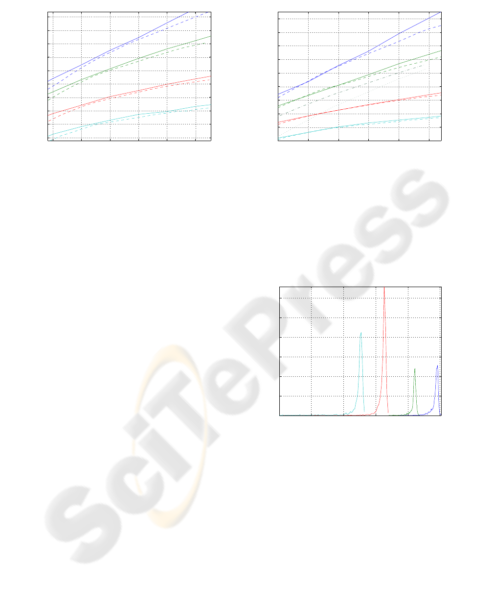
5 10 15 20 25 30
24
26
28
30
32
34
36
38
40
42
CSNR(dB)
PSNR(dB)
Figure 3: Performance of proposed system (dashed) com-
pared to reference system (solid). “Goldhill” image. r
avg
in
channel samples/pixel, from below: 0.03, 0.1, 0.3, 0.5.
rates (bit/channel symbol), each assumed to achieve
AWGN capacity for a given CSNR. To further max-
imize the average spectral efficiency (ASE) continu-
ous power adaptation to is used within each CSNR
region (Gjendemsjø et al., 2005).
The examples of the proposed coder are given for a
certain CSNR, (¯γ), and an overall target compression-
rate, r
avg
(channel samples/pixel). To be able to
compare with the reference system, a bitrate in
bits/channel sample, R
c
, is found for a given ¯γ for
the channel code, and the resulting source bitrate, R
s
,
in bits/pixel is found and given as a parameter to the
reference image coder through
R
s
= r
avg
R
c
. (17)
4 RESULTS
The following results are for images transmitted over
a Rayleigh fading channel. The Doppler frequency is
set to f
d
= 100 Hz, and the carrier frequency, f
c
, is
set to 2 GHz, resulting in a mobile velocity of 15 m/s.
The channel is simulated according to the Jakes’ cor-
relation model (Jakes, 1974). The number of channel
states with transmission, M, is set to four for the pro-
posed system and the reference system, thus allowing
one outage state for both cases.
The quality of the received image is measured by
peak signal-to-noise ratio (PSNR), defined as the ra-
tio between the squared maximum pixel value, and
the mean squared error (MSE) on a pixel basis for the
whole image.
From Figure 3 and Figure 4 we see that the pro-
posed system performs slightly poorer compared to
the reference system. When comparing the two sys-
tems, it is however important to remember that the
reference system uses near capacity achieving chan-
5 10 15 20 25 30
20
22
24
26
28
30
32
34
36
38
CSNR(dB)
PSNR(dB)
Figure 4: Performance of proposed system (dashed) com-
pared to reference system (solid). “Bridge” image. r
avg
in
channel sample/pixel, from below: 0.03, 0.1, 0.3, 0.5. Pro-
posed system for r
avg
= 0.3 with channel information every
1000’th (dash-dotted), and 20000’th channel symbol (dot-
ted).
nel transmission. In practice the reference system
would require infinite complexity and infinite delay.
Looking at robustness we can see from Figure 5, that
20 25 30 35 40
0
0.05
0.1
0.15
0.2
0.25
0.3
PSNR (dB)
p (PSNR)
Figure 5: Estimated distributions of PSNR for target aver-
age rate r
avg
, from left: 0.03, 0.1, 0.3, 0.5. For ¯γ = 22 dB.
“Goldhill” image.
even without any error protecting or correcting code,
the robustness in the proposed system is quite high.
Where as the reference channel transmission system
will break down without perfect channel knowledge,
the proposed system degrades gradually. In Figure 4,
we have included the case where the transmitter does
not have perfect channel knowledge. Two cases are
included, one where the transmitter only knows the
channel state for every 1000’th channel symbol, and
one for every 20000’th symbol. For r
avg
= 0.3 the
total number of channel symbols is about 78300 for a
512 × 512 image. We will however not analyze this
any further in this paper. It should noted that the ref-

erence system uses an optimal threshold for outage,
while the proposed system uses a fixed outage thresh-
old of ˆγ
1
= 2 for simplicity.
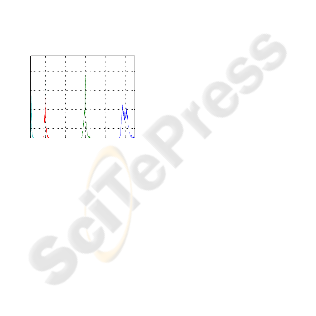
It should be emphasized that the performance for
the proposed system is an average. Due to the limited
number of symbols needed to transmit an image, the
channel will not be fully ergodic. The result of this
can be seen in the distribution of the average rate r
avg
in Figure 6. The assumed rate is based on the preal-
location of the blocks, but since the probabilities of
each channel state will vary, the number of channel
symbols will also vary. Since r
avg
varies, the actual
CSNR will vary slightly as well. So when reading the
results in Figure 3 and Figure 4, one should keep in
mind that the CSNR and PSNR is plotted as an aver-
age. An estimated distributions of the PSNR for dif-
ferent r
avg
is given in Figure 5.
0.1 0.2 0.3 0.4 0.5
0
0.01
0.02
0.03
0.04
0.05
0.06
0.07
0.08
r
avg
p (r
avg
)
Figure 6: Estimated distributions of average trans-
mission rates r
avg
for target average rate from left:
0.03, 0.1, 0.3, 0.5. For ¯γ = 22 dB. “Goldhill” image.
In Figure 3 and Figure 4, it can be seen that the per-
formance of the proposed coder is not parallel with
the performance of the reference coder. For high
CSNR values this is due to the number of mapping
rates available is to low in the rate-range of 0 to 2.
For low CSNR values, there is a need for mappings
with rates higher than 2.
5 CONCLUSION
We have shown how a joint source channel image
coder system can achieve robust performance for
transmission over a Rayleigh fading channel, when
allowing the average rate to vary slightly around a tar-
get rate. This is done by choosing nonlinear mappings
best suited for the current channel condition, the im-
portance of the transmitted image block, and by allo-
cating the power to minimize the distortion. The pro-
posed system has been shown to be comparable to a
reference tandem system using capacity-approaching
codes.
REFERENCES
Balasingham, I. (1998). On Optimal Perfect Reconstruc-
tion Filter Banks for Image Compression. PhD the-
sis, Norwegian University of Science and Technology,
Norway.
Berger, T. (1971). Rate Distortion Theory: A Mathematical
Basis for Data Compression. Prentice Hall, Engle-
wood Cliffs, NJ.
Coward, H. and Ramstad, T. (2000). Robust image com-
munication using bandwidth reducing and expand-
ing mappings. volume 2, pages 1384–1388, Pacific
Grove, CA, USA. Conf. Record 34th Asilomar Conf.
Signals, Syst., Comput.
Fuldseth, A. and Ramstad, T. A. (1997). Bandwidth com-
pression for continuous amplitude channels based on
vector approximation to a continuous subset of the
source signal space. In Proc. IEEE Int. Conf. on
Acoustics, Speech, and Signal Proc. (ICASSP), vol-
ume 4, pages 3093–3096.
Gersho, A. and M. Gray, R. (1992). Vector Quantization
and Signal Compression. Kluwer Academic Publish-
ers, Boston, MA, USA.
Gjendemsjø, A., Øien, G. E., and Holm, H. (2005). Op-
timal power control for discrete-rate link adaptation
schemes with capacity-approaching coding. In Proc.
IEEE Global Telecommunications Conference, pages
3498–3502, St. Louis, MO.
Holm, H., Øien, G. E., Alouini, M.-S., Gesbert, D., and
Hole, K. J. (2003). Optimal design of adaptive coded
modulation schemes for maximum spectral efficiency.
pages 403–407. Proc. Signal Processing Advances in
Wireless Communications (SPAWC).
Jakes, W. C. (1974). Microwave Mobile Communication.
Wiley, New York.
Lervik, J. M. and Ramstad, T. A. (1996). Optimality of mul-
tiple entropy coder systems for nonstationary sources
modeled by a mixture distribution. In Proc. IEEE
Int. Conf. on Acoustics, Speech, and Signal Proc.
(ICASSP), volume 4, pages 875–878, Atlanta, GA,
USA. IEEE.
Mittal, U. and Phamdo, N. (2002). Hybrid digital-
analog(hda) joint source-channel codes for broadcast-
ing and robust communication. IEEE Trans. Inform.
Theory, 48(5):1082–1102.
Shannon, C. E. (1948). A mathematical theory of commu-
nication. Bell Syst. Tech. J., 27:379–423.
Tanabe, N. and Farvardin, N. (1992). Subband image cod-
ing using entropy-coded quantization over noisy chan-
nels. IEEE J. Select. Areas Commun., 10(5):926–943.
Taubman, D. and Marcellin, M. (2001). JPEG2000 Im-
age compression fundamentals, standards and prac-
tice. Kluwer Academic Publishers.