
SEGMENTING OF RECORDED LECTURE VIDEOS
The Algorithm VoiceSeg
Stephan Repp, Christoph Meinel
Hasso-Plattner-Institut for Software System Engineering (HPI),University of Potsdam, D-14440 Potsdam, Germany
Keywords: Topic segmentation, recorded lecture videos, imperfect and erroneous transcripts, indexing, retrieval.
Abstract: In the past decade, we have witnessed a dramatic increase in the availability of online academic lecture
videos. There are technical problems in the use of recorded lectures for learning: the problem of easy access
to the multimedia lecture video content and the problem of finding the semantically appropriate information
very quickly. The first step to a semantic lecture-browser is the segmenting of the large video-corpus into a
smaller cohesion area. The task of breaking documents into topically coherent subparts is called topic
segmentation. In this paper, we present a segmenting algorithm for recorded lecture videos based on their
imperfect transcripts. The recorded lectures are transcripted by an out-of-the-box speech recognition
software with a accuracy of approximately 70%-80%. Words as well as a time stamp for each word are
stored in a database. This data acts as the input to our algorithm. We will show that the clustering of similar
words, the generation of vectors with the values from the clusters and the calculation of the cosine-mass of
adjacent vectors, leads to a better segmenting result compared to a standard algorithm.
1 INTRODUCTION
This paper describes a technique for improving
access to recorded lecture videos by dividing them
into topically coherent sections without the help of
extern resources like slides or textbooks. The aim of
this paper is to discover the topic boundaries of the
lecture videos based on the imperfect transcripts of
the recorded lecture videos. Segmenting of the
lecture is important for further processing of the
data. Topic segmentation has been extensively used
in information retrieval and text summarization. For
the information retrieval task, the user would prefer
a document passage in which the occurrence of the
word/topic is concentrated in one or two passages.
Further more, these elements of the lecture are
necessary for the index in a semantical design (Repp
and Meinel, 2006).
In the past decade, we have witnessed a
dramatic increase in the availability of online and
offline academic lecture material. An example of
this being, the newly developed tele-teaching system
called "tele-Task" (Schillings et al., 2002). This
system allows a video sequence to be bundled with
the capture of the speaker’s desktop. This
multimedia stream can be broadcast live or on
demand over the Internet. These archived
educational resources can potentially change the
way people learn (Linckels, et. al. 2005).
Transcripts of live-recorded lectures consist of
unscripted and spontaneous speech. Thus, lecture
data has much in common with casual or natural
speech data, including false starts, extraneous filler
words and non-lexical filled pauses (Glass et al.,
2004). Furthermore, a transcript is a stream of words
without punctuation marks. Of course, there is also a
great variation between one tutor’s speech and
another’s. One may speaks accurately, the next
completely differently with many grammatical
errors, for example. One can also easily observe that
the colloquial nature of the data is dramatically
different in style from the same presentation of this
material in a textbook. In other words, the textual
format is typically more concise and better
organized. Speech recognition software produces
outcomes prone to error, approximately 20%-30% of
the detected words being incorrect. The not-in-the-
vocabulary-problem is a dilemma of the recognition
software too (Hürst, 2003). The software needs a
database of all words used by the lecturer for the
transcription process. If a word that occurs in the
speech of the lecturer is not in the vocabulary, the
wrong word is transcripted by the engine.
Furthermore, the changing of language in a
presentation may lead the software to unsolvable
317
Repp S. and Meinel C. (2006).
SEGMENTING OF RECORDED LECTURE VIDEOS - The Algorithm VoiceSeg.
In Proceedings of the International Conference on Signal Processing and Multimedia Applications, pages 317-322
DOI: 10.5220/0001570603170322
Copyright
c
SciTePress

problems. A lecture presented in German may
sometimes use English terminology. This causes
wrong words to be included in the transcript
Our algorithm takes these properties into
account, and in this paper, we will show how our
segmenting technique will work.
2 RELATED WORK
In the past decade, a lot of research on topic
segmentation has been carried out. In (Reynar,
1998), Reynar gives a thorough review of Topic
Segmentation. The algorithm TextTiling (Hearst,
1997) and Dotplotting (Reynar, 1998) are based on
lexical item repetition (an item being a sequence of
characters, a stem, a morphological root or an
ngram). Another emphasis of research is the area
based on Semantic Network (Morris and Hirst,
1991) and (Nicola, 2004). Morris used a thesaurus to
detect topic boundaries based on lexical cohesion
relations called lexical chains. An application of text
segmentation is the segmentation of broadcast news.
This application uses systems relying on supervised
learning (Beefermann et. al., 1999). These
approaches cannot be applied to domains for which
no training data exists.
The third main research focus is to detect patterns
(for instance cue phrases) around topic boundaries
(Chau et. al., 2004)(Tür et. al., 2001). They use the
appearance of particular words before a boundary
and the appearance of cue words at the beginning of
the previous sentence. Chau et. al. combined and
adapted the TextTiling technique, the cue phrase
technique and the lexical cohesion technique to
perfect transcripted lecture videos. He obtained a
segmenting result of around 70% precision and
around 70% recall. This research was done for
perfect text or transcript with whole sentence and
correct grammar.
These techniques require an accurate corpus of
text! As the author knows, no work is done to do the
topic segmenting with real world data from
imperfect transcript of recorded lectures and without
other resources like textbooks or slides. In this
paper, we will demonstrate some results of our
research on the topic of segmentation of imperfect
transcripts.
The indexing-process resulting in the imperfect
transcript of lecture videos is described in (Hürst,
2003). He evaluated that indexing may be done with
a high vocabulary automatic speech recognition
system (a commercial, “out-of-the-box” system).
However, the accuracy of the speech recognition
software is rather low, the recognition accuracy of
audio lecture being approximately 22%-60%. It is
shown in (Chau et. al., 2004) that audio retrieval can
be performed with out-of-the-box speech recognition
software. Hürst comes to the conclusion that the
imperfect transcripts of recorded lectures are useful
for further standard indexing processes (Hürst,
2003). Repp and Meinel show that a smart
semantical indexing may be done even with
incorrect transcripts (Repp and Meinel, 2006).
To segment the lecture, the chapter from the
slides is often used (Hürst et. al., 2003). However,
the segments of the slides are partially wrong,
because the lecture speech is highly dynamics. The
tutor uses his freedom to report on topics not
classified by the slides.
3 ALGORITHM
An algorithm which detects topic boundaries in
imperfect transcripts has to be very robust against
wrongly recognized words, and to the not-in-the-
vocabulary-problem. Furthermore, the transcripts
consist of a stream of words and not of cohesive
areas like sentences or chapters. We show in our
algorithm VoiceSeg how topic-boundaries for
domain independent and imperfect transcripts of
recorded lecture videos can be generated. In addition
we implement a TextTiling algorithm for comparing
our algorithm with a standard segmenting algorithm.
Our VoiceSeg algorithm consists of five steps: After
a standardized preprocessing with a ‘tagger’ and
deletion of stop-words, the similar and adjacent
words are grouped in clusters. We fill the vector-
elements with the values of the cluster data. After
that we build vectors and weight the elements in the
vector. Then we calculate the cosine-mass of two
adjacent vectors to get the similarity of the
neighboring areas. The last step involves the
determining of boundaries.
3.1 Preprocessing
First the stop-words from the output transcript of the
out-of-the-box speech recognition software are
deleted. The generation of the transcript is described
in (Repp and Meinel, 2006). After that, the words
from the transcript are transformed into their stem
with the TreeTagger provided by the institute for
“Maschinelle Sprachverarbeitung, Stuttgart”
(http://www.ims.uni-stuttgart.de; last access:
02/02/2006). The transcript is now a stream of stems
with a time stamp for each stem.
SIGMAP 2006 - INTERNATIONAL CONFERENCE ON SIGNAL PROCESSING AND MULTIMEDIA
APPLICATIONS
318
This stream can contain all verbosity, such as a
noun, verb, number etc… From that set we store the
distinct stems
R
L
.
(1)
In other words,
R
L consist of all distinct stems
(without stop-words) detected by the speech
recognition engine of the course. A term is any
stemmed word within the course.
3.2 Clustering
The clustering is used to detect cohesive areas
(lexical chains) in the transcript. Our algorithm is
similar to the algorithm descript in (Galley et. al.,
2003), but we generated windows after a fix time
interval.
A chain is constructed to consist of all repetitions
ranging from the first to the last appearance of the
term in the course. The chain is divided into subparts
when there is a long hiatus (time distance ε )
between the terms. The chain is a segment of
accumulated appearance of equal words w
i
R
L
∈
inside the transcript. For all term-chains with start
time and end time are generated. The chains of the
terms may be overlap, because they have been
generated for any stems used in the course. For all
chains (we will call them a cluster) that have been
identified for the terms, a weighting scheme is used.
Clusters containing more repeated terms receive
higher scores.
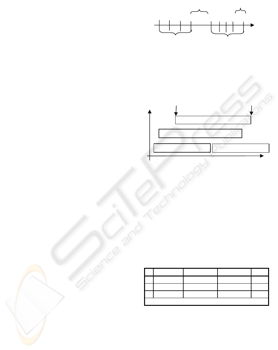
Let ts
∈N be the start-time and te∈N be the end-
time of a term. Every occurrence of the term
w
i
in
the transcript has a start-time ts
p
and an end-time te
p
.
Let p
∈N be the position of the term w
i.
p=1 is the
first occurrence of the term w
i
, p=2 is the second
occurrence of w
i
, p=E is the last occurrence of w
i
in
the stream. The term w
i
on the position p is then
defined as w
i,p
. (see Figure 1) Let ε be the maximum
time distance between two equal terms (w
i,p
.and
w
i,p+1
) inside of a cluster. Let TN be the number of
the terms w
i
inside of the cluster. Let n be the index
of TN. Thus the cluster is defined as:
where for all:
and:
and: (2)
p=E-TN+1 is the first position of the term w
i
inside
the last cluster (of w
i
) in the course.
Figure 1: The clusters for one example word w
i
.
A cluster is an area inside the course. A term w
i
occurs very often in this area and the time distance
between adjacent and equal terms in this area is
lower than the bound ε. The clusters are generated
for all w
i..
w
i
w
3
w
2
w
1
time
Figure 2: Stored data for the cluster.
The main steps of the clustering algorithm of the
course run in the following way (see the equation (3)
and (4)): Take the term w
i
and create the clusters C
k
so that the distance between two equal terms
(w
i,p
.and w
i,p+1
) is not more than the time-distance ε,
otherwise create a new cluster C
k+1
. Count the
occurrence TN
k
of the terms w
i
in the cluster C
k
and
store TN
k
, the start-time and the end-time of C
k
in
the database (see Figure 2 and Table 1). Do this for
all terms w
i.
.
Table 1: Example set of cluster-data.
pp
tets
−
>
+1
ε
(3)
→ w
i,p+1
is in the cluster C
k
pp
tets −≤
+1
ε
(4)
→ w
i,p+1
is not in the cluster C
k
; start a new cluster
C
k+1
The tables 2 and table 3 provide overview of the
index and some important abbreviations used in this
paper.
C Term start-time end-time TN
1 TCP 160sec 240sec 15
2 TCP 250sec 360sec 4
3 topology 152sec 260sec 7
etc…
w
i,5
w
i,6
w
i,7
w
w
w
i,1
w
i,2
w
i,3
ts
9
-te
8
≤ ε
ts
5
-te
4
> ε
cluster
k
cluster k+1
()( )( )
{}
TN
TNpTNpTNpipppipppi
tetswtetswtetswC
111,
2
111,
1
,
,,,...,,,,,,
−+−+−++++
=
C
1
,w
1
:TCP, TN
1
: 15
star
t
-time en
d
-time
C
2,
w
1
:TCP, TN
2
: 4
C
3
,w
2
: topology, TN
3
: 7
C
4
, w
3
:WWW, TN
4
: 3
},...,,,{
321 iR
wwwwL =
10 −<≤ TNn
11 +
−
≤≤ TNEp
ε
≤−
+++
)(
1 npnp
tets
SEGMENTING OF RECORDED LECTURE VIDEOS - The Algorithm VoiceSeg
319
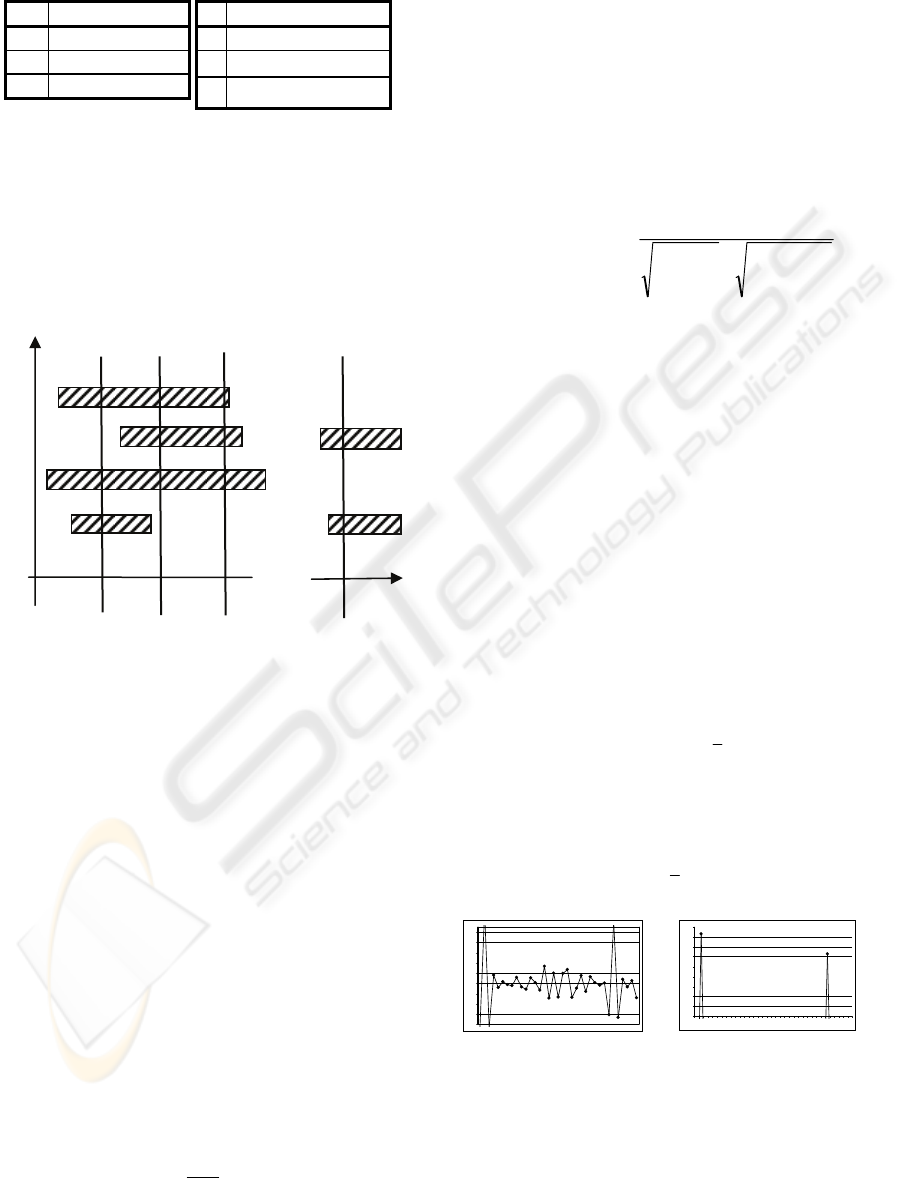
Table 2: Abbreviation. Table 3: Overview of
used indices
.
3.3 Vectoring and Weighting
The next step is to produce the vectors. In order to
do so, we use the cluster-values at a specific time
j
t to create the vector a
j
. Furthermore, we define a
time-distance d between two adjacent vectors (see
equation (5)). After the time d we produce a new
vector a
j+1
: dtt
jj
+=
+1
(5)
w
i
…
w
4
…
w
3
…
w
2
…
w
1
…
time
a
1
a
2
a
3
a
j
Figure 3: The production of the vectors.
The elements a
j,i
are filled with the term number
(TN
k
) from the cluster. When there is no cluster for a
word w
i
and for the specific time
j
t
the element a
j,i
is filled with 0. The figure 3 shows this procedure.
We define a parameter WM as a minimum term
number needed in the cluster for filling the element
a
j,i
. WM may, for example, be defined as 3. If the
cluster consists of a term number TN
k
which is
higher or equal than 3 aj,i is filled with TN
k
,
otherwise aj,i is set to 0.
We assume that a topic shift occurs, if somebody
uses different terms. The lecturer speaks on the topic
a, than topic b, than topic c and so on. He used for
each topic some different terms. A topic shift arises,
if a term occurs only in few chains. So the weighting
of the elements works in the following way: If a
cluster occurs very infrequently it is much more
relevant than the clusters which occur very often.
The cluster is also more relevant, if the TN
k
is high.
So the elements are weighted as follows:
(6)
where n
i
= is the number of all clusters for the term
w
i
in the course. (a
j,i
was filled with TN
k
as
described
before).
3.4 Similar Measuring
For the similar measuring we use the well known
cosine-mass method (Baeza-Yates and Ribeiro-Neto,
1999). The calculation of the cosine-mass of
adjacent vectors is defined as:
(7)
The elements S
0
and S
j
are represented by 0 for the
reason that no values of neighboring vectors exist.
3.5 Identifying Boundaries
Our identification of the boundaries is based on
(Hearst, 1997). The calculation of the equation (8)
produces a similarity graph. For better understanding
of the variation of S
j
score, each time its value goes
from a high value to a low value and back up to high
again, the resulting valley is called a downhill. The
deeper the downhill, the better the hit for a
boundary. The downhill is defined as:
jjjjj
SSSSSdownhill −+
−
=
+− 11
)( (8)
We calculate all downhills with the equation above
(8) and get the following graph, which is shown by
the figure 4. Once all downhills in the data-set have
been calculated, their mean
x and the standard
deviation
σ
of the set of )(
j
Sdownhill are
evaluated. The topic-boundaries are elected if the
data satisfies the constraint expressed in equation
(9). See figure 5.
σ
+≥ xSdownhill
j
)(
(9)
Figure 4: The downhills. Figure 5: Detecting of
segment boundaries.
In the result-set of potential boundaries, we may
detect values which are very close to each other. If
this occurs and the densely populated results ensue,
w stem
a vector
C cluster
TN term number in C
i number of the stem
k number of the cluster
p position of the term
j number of the Vector
∑∑
∑
=
+
=
=
+
++
×
×
==
m
i
ij
m
i
ji
m
i
ijji
jjj
aa
aa
aasimS
1
2
,1
1
2
1
,1
11
)()(
),(
i
ij
ij
n
a
a
,
,
=
0,57
0,67
0,77
0,87
0,97
1,07
1,17
1,27
1,37
1,47
2,5 4 5,5 7 8, 5 10
-0,8
-0,6
-0,4
-0,2
0
0,2
0,4
0,6
0,8
1
SIGMAP 2006 - INTERNATIONAL CONFERENCE ON SIGNAL PROCESSING AND MULTIMEDIA
APPLICATIONS
320

then data may be cancelled. If the distance between
two neighboring boundaries S
j
and S
j+n
is lower than
60 sec the boundary S
j+n
is not a boundary and it is
cancelled.
It must be borne in mind that the algorithm detects
the similarity between two adjacent vectors, which
have a time distance of d. So the start time of a topic
segment falls at the calculated time (
j
t ) minus the
distance d. The start time of the topic segment is,
therefore,
1−j
t
.
4 EVALUATION
The corpus of the videos consists of the course
“Einführung in das WWW” held in German in the
first semester 2005 at the Hasso Plattner Institut
Potsdam. The videos can be found at www.tele-
task.de. This part of the course consists of 16
lectures, each lecture lasting approximately 90
minutes. The video corpus has a total length of
approximately 1440 minutes. As previously
mentioned the word error rate is between 20%-30%.
Our algorithm is based on the imperfect transcript
of recorded videos. It is very difficult to compare
our algorithm with other reference data sets, because
no such sample sets exist for this purpose.
There stile exists the sizeable problem of hitting
the manual segmenting area with the help of a
segmenting algorithm. If we decide that the segment
starts at one particular time it is not possible to hit
the boundary in exact seconds by a segmenting
algorithm. Therefore, the so-called start-duration
area is determined at the beginning of a segment.
This start-duration area is an area (start-time to start-
time + start-duration), where the topic starts. If the
auditor begins the topic in this area, he may
understand the whole topic. For instance, the speaker
starts with a short general introduction, and then
begins the segment “topology”. All hits in that
beginning-phase (start-duration phase) are taken as
correct hits. Furthermore a variation of ± 15sec of
this area is accepted.
We can not use the probabilistic accuracy metric
(Beeferman et. al., 1999) for topic segmentation
because the mass is based on sentence and an exact
defined boundary. In our case we have an area of a
break, which we mention before. For our evaluation
we use the recall and precision mass adapted to topic
segmentation (Baeza-Yates and Ribeiro-Neto,
1999), (Chau et. al.,2004).
We manually segment tree lectures of the course
with 77 segments. A simple baseline segmenting
algorithm is also developed. Given the average
distance (d
b
) between two adjacent segments in the
lecture, the baseline algorithm chooses every point
(after the time d
b
) to represent a boundary.
The TextTiling algorithm is based on (Hearst,
1997) and (Chau et. al., 2004). We build a sliding
window system. We move a sliding window (e.g.
120 words) across the text-stream over a certain
interval (e.g. 20 words) and compare the
neighboring windows with each other. The equation
(7) is used to calculate the similarity between the
vectors. The boundaries identification is done in the
same way as it is done by the VoiceSeg algorithm.
If you are interested in the detailed evaluation of
the data please contact the author.
Table 4: Baseline uniformly distributed.
baseline precision recall
120 / 10 32.50% 33.66%
Table 5: TextTiling variation of the step size.
window / step precision recall
120 / 10 36.07% 28.57%
120 / 20 38.20% 23.38%
120 / 30 35.00% 18.18%
Table 6: TextTiling variation of the window size.
window / step precision recall
140 / 20 37.84% 18.18%
120 / 20 38.30% 23.38%
100 / 20 33.96% 23.38%
Table 7: VoiceSeg variation of the cluster number TN;
parameters:
ε
=120 second, d=15 second.
word in cluster TN precision recall
min 1 54.05% 51.95%
min 2 65.75% 62.38%
min 3 54.88% 58.44%
min 4 51.39% 48.05%
min 5 55.07% 49.35%
Table 8: VoiceSeg variation of the vector distance d;
parameters:
ε
=120 second, TN=2.
vector distance d precision recall
5 sec 45.31% 37.66%
10 sec 51.39% 48.05%
15 sec 65.75% 62.38%
20 sec 59.21% 58.44%
25 sec 66.18% 58.44%
30 sec 62.90% 50.65%
45 sec 56.67% 44.16%
60 sec 61.70% 37.66%
90 sec 53.13% 22.08%
SEGMENTING OF RECORDED LECTURE VIDEOS - The Algorithm VoiceSeg
321

Table 9: VoiceSeg variation of the cluster parameter
ε
;
parameters: d=15 second, TN=2.
cluster distance
ε
precision recall
60 sec 42.39% 50.65%
120 sec 65.75% 62.38%
180 sec 45.95% 44.38%
240 sec 46.27% 40.28%
300 sec 46.23% 33.77%
5 CONCLUSION AND OUTLOOK
In this paper, we present a system of segmenting
imperfect transcripted lecture videos. We show in our
evaluation that it is possible to detect boundaries in an
imperfect transcript. The results are surprisingly high.
Bear in mind that the raw material is highly erroneous
(only 70%-80% being correctly recognized). The
parameter d=15 seconds,
ε
=120 seconds and a TN of
2 are considered optimum. The VoiceSeg algorithm
(precision 65.75%, recall 62.38%) is more
successful at detecting the boundaries compared to
the adapted TextTiling-algorithm (precision 38.30%,
recall 23.38%) and the baseline algorithm (precision
32.50%, recall 33.66%).
Our Algorithm and the TextTiling-algorithm have
problems in detecting boundaries inside repetition-
segments or inside overview-segments (which occur at
the beginning and end of a lecture). In these segments,
many infrequent words occur very close together.
Further study may be carried out with our new
algorithm VoiceSeg. We will study the influence of
difference weighting equations and the influence of
other cluster values (length, correlation, etc…) to the
results. We will adapt the cue phrase, or other pattern
detecting techniques in the areas around potential
boundaries (for example, pauses). Another important
point is to compare our result with the result of other
state of the art topic segmentation algorithm (Galley
et. al., 2003), (Choi 2000) using erroneous transcripts.
We are also working on a "lecture-browser" for a
simple navigation through the corpus of lectures. This
lecture-browser will help students in their learning and
will make the process of learning more efficient. The
combination of pedagogical and content description
leads to novel forms of visualization and exploration
of course lectures.
REFERENCES
Schillings V.; Meinel, C., 2002. tele-TASK - Teleteaching
Anywhere Solution Kit. In Proceedings. ACM
SIGUCCS 2002, 130-133. Providence, USA.
Hürst, W., 2003. A qualitative study towards using large
vocabulary automatic speech recognition to index
recorded presentations for search and access over the
web. IADIS International Journal on WWW/Internet,
Volume I, Number 1: 43-58.
Chau, M.; Jay, F.; Nunamaker, Jr.; Ming, L., Chen, H.
,2004. Segmentation of Lecture Videos Based on Text:
A Method Combining Multiple Linguistic Features. In
Proceedings of the 37th Hawaii International
Conference on System Sciences. Hawaii, USA.
Baeza-Yates, R.; Ribeiro-Neto, B., 1999. Modern
Information Retrieval. New York, USA: Addison-
Wesley.
Glass, J.; Hazen, T.J.; Hetherington, L.; Wang, C., 2004.
Analysis and Processing of Lecture Audio Data:
Preliminary Investigations. In Proceedings of the
HLT-NAACL 2004 Workshop on Interdisciplinary
Approaches to Speech Indexing and Retrieval, 9-12.
Boston, MA, USA.
Linckels, S.; Meinel, Ch.; Engel, T., 2005. Teaching in
theCyber Age: Technologies, Experiments, and
Realizations. In Proceedings of 3. Deutschen e-
Learning Fachtagung der Gesellschaft für Informatik
(DeLFI), 225 – 236. Rostock, Germany.
Repp, S.; Meinel, C., 2006. Semantic Indexing for
Recorded Educational Lecture Videos. In Proceedings
of the Fourth Annual IEEE International Conference
on Pervasive Computing and Communications
Workshops (PERCOMW'06), 240-245. Pisa, Italy.
Nicola, S., 2004. Applications of Lexical Cohesion
Analysis in the Topic Detection and Tracking Domain.
Ph.D. diss., Dept. of Computer Science, University
College Dublin.
Hearst, Marti A., 1997. TextTiling: Segmenting Text into
Multi-paragraph Subtopic Passages. Computational
Linguistics 23, 33-64. Cambridge, MA: MIT Press.
Reynar, J. C., 1998. Topic Segmentation: Algorithms and
application. Ph.D. diss., University of Pennsylvania.
Morris, J.; Hirst, G., 1991. Lexical cohesion computed by
thesaural relations as an indicator of the structure of
text. Computational Linguistics 17, 21-48. Cambridge,
MA: MIT Press.
Tür, G; Hakkani-Tür, D; Shriberg, E., 2001. Integrating
Prosodic and Lexical Cues for Automatic Topic. In
Segmentation CoRR
Beeferman, D; Adam, L.; Berger, A.; Lafferty, J., 1999.
Statistical Models for Text Segmentation. In Machine
Learning 34
Choi, F., 2000. Advance in domain independent linear text
segmentation. In Proceedings of NAACL
Galley, M.; McKeown, K.; Fosler-Lussier, E.; Jing, H.,
2003. Discourse Segmentation of Multi-Party
Conversation In Proceedings of the 41st Annual
Meeting of the Association for Computational
Linguistics
SIGMAP 2006 - INTERNATIONAL CONFERENCE ON SIGNAL PROCESSING AND MULTIMEDIA
APPLICATIONS
322
