
EVALUATING THE POTENTIAL OF CLUSTERING
TECHNIQUES FOR 3D OBJECT EXTRACTION FROM LIDAR
DATA
Farhad Samadzadegan, Mehdi Maboodi, Sara Saeedi, Ahmad Javaheri
Department of Geomatics Engineeering, University of Tehran, Tehran, Iran
Keywords: Clustering, LIDAR, K-Mean, FCM, SOM, Filtering, 3D Objects.
Abstract: During the last decade airborne laser scanning (LIDAR) has become a mature technology which is now
widely accepted for 3D data collection. Nevertheless, these systems have the disadvantage of not
representing the desirable bare terrain, but the visible surface including vegetation and buildings. To
generate high quality bare terrain using LIDAR data, the most important and difficult step is filtering, where
non-terrain 3D objects such as buildings and trees are eliminated while keeping terrain points for quality
digital terrain modelling. The main goal of this paper is to investigate and compare the potential of
procedures for clustering of LIDAR data for 3D object extraction. The study aims at a comparison of K-
Means clustering, SOM and Fuzzy C-Means clustering applied on range laser images. For evaluating the
potential of each technique, the confusion matrix concept is employed and the accuracy evaluation is done
qualitatively and quantitatively.
1 INTRODUCTION
In recent years LIDAR data has become as a highly
acknowledged data source for interactive mapping
of 3D man-made and natural objects from the
physical earth’s surface. The dense and accurate
recording of surface points has encouraged research
in processing and analysing the data to develop
automated processes for feature extraction, object
recognition and object reconstruction. However, the
algorithm for segmentation of this kind of data, i.e.
distinguish between ground surface and objects on
the surface, is still on going researched (Haala and
Brenner 1999; Axelsson, 1999; Maas and
Vosselman, 2001).
Nowadays, laser-scanning systems are able to
collect of two different types from the ground
surface and the objects over it; first-pulse and last-
pulse data. Laser pulses have one important
advantage that partially they penetrate the vegetation
in gaps between leaves and obtain data reflected
from points underneath the vegetation. This property
of the laser defines the difference between first- and
last- pulse data. That means in first-pulse data, the
data of the vegetation’s surface is available, while it
is not the case in last-pulse. The other main property
of laser scanning systems is the ability to provide the
range data from the objects in addition to the
reflectance image data (intensity data). This range
data obtained from the elevation points over the
earth’s surface or other 3D objects can be converted
to a digital range image. Therefore the laser
scanners, nowadays, can provide both range image
and intensity image in two different types, first- and
last-pulse data (Sithole, 2003; Roggero, 2002).
The paper shows the potential of the analysis of
height texture for the automatic segmentation of
LIDAR regular range datasets and 3D objects
extraction in the segmented data. Based on the
definition and computation of a number of texture
measures used as bands in three clustering
approaches (i.e. K-Mean, FCM and SOM), 3D
objects like buildings and trees can be recognized
from bare terrain.
2 CLUSTERING OF LIDAR DATA
Cluster analysis is a difficult problem because many
factors (such as effective similarity measures,
criterion functions, algorithms and initial conditions)
come into play in devising a well tuned clustering
149
Samadzadegan F., Maboodi M., Saeedi S. and Javaheri A. (2006).
EVALUATING THE POTENTIAL OF CLUSTERING TECHNIQUES FOR 3D OBJECT EXTRACTION FROM LIDAR DATA.
In Proceedings of the First International Conference on Computer Vision Theory and Applications, pages 149-154
DOI: 10.5220/0001378301490154
Copyright
c
SciTePress

technique for a given clustering problem. Cluster
analysis is an unsupervised learning method that
constitutes a cornerstone of an intelligent data
analysis process. It is used for the exploration of
inter-relationships among a collection of patterns, by
organizing them into homogeneous clusters. It is
called unsupervised learning because unlike
classification (known as supervised learning), no a
priori labeling of some patterns is available to use in
categorizing others and inferring the cluster structure
of the whole data. Intra-connectivity is a measure of
the density of connections between the instances of a
single cluster. A high intra-connectivity indicates a
good clustering arrangement because the instances
grouped within the same cluster are highly
dependent on each other. Inter-connectivity is a
measure of the connectivity between distinct
clusters. A low degree of interconnectivity is
desirable because it indicates that individual clusters
are largely independent of each other.
K-Means: The most well-known partitioning
algorithm is the K-Means (
Rottensteiner and Briese,
2002
). The K-Means method partitions the data set
into k subsets such that all points in a given subset
are closest to the same centre. In detail, it randomly
selects k of the instances to represent the clusters.
Based on the selected attributes, all remaining
instances are assigned to their closer centre. K-
Means then computes the new centres by taking the
mean of all data points belonging to the same
cluster. The operation is iterated until there is no
change in the gravity centres. If k cannot be known
ahead of time, various values of k can be evaluated
until the most suitable one is found. The
effectiveness of this method as well as of others
relies heavily on the objective function used in
measuring the distance between instances. The
difficulty is in finding a distance measure that works
well with all types of data.
FCM: Traditional K-Means clustering
approaches generate partitions; in a partition, each
pattern belongs to one and only one cluster. Hence,
the clusters in a hard clustering are disjoint. Fuzzy
clustering extends this notion to associate each
pattern with every cluster using a membership
function. Larger membership values indicate higher
confidence in the assignment of the pattern to the
cluster. One widely used algorithm is the Fuzzy C-
Means (FCM) algorithm, which is based on K-
Means. FCM attempts to find the most characteristic
point in each cluster, which can be considered as the
“centre” of the cluster and, then, the grade of
membership for each instance in the clusters.
Let us assume as a Fuzzy C-Means Functional
where,
[
]
{
}
cjyY
j
,1∈= is the set of centers of
clusters;
)(
kj
xE is a dissimilarity measure (distance
or cost) between the sample
j
x and the center
j
y
of a specific cluster j; U = [u
jk
] is the c × n fuzzy c-
partition matrix, containing the membership values
of all samples in all clusters;
),1[ ∞∈m
is a control
parameter of fuzziness.
∑∑
==
=
n
k
c
j
kj
m
jkm
xEuYUJ
11
)()(),(
(1)
The clustering problem can be defined as the
minimization of J
m
with respect to Y, under the
probabilistic constraint:
1
1
=
∑
=
c
j
jk
u
(2)
The Fuzzy C-Means algorithm consists in the
iteration of the following formulas:
()
()
∑
∑
=
=
=
n
k
m
jk
c
j
k
m
jk
j
u
xu
y
1
1
for all j, (3)
⎪
⎪
⎭
⎪
⎪
⎬
⎫
⎪
⎪
⎩
⎪
⎪
⎨
⎧
≠∀=
∀〉
⎟
⎟
⎟
⎠
⎞
⎜
⎜
⎜
⎝
⎛
⎟
⎟
⎠
⎞
⎜
⎜
⎝
⎛
=
−
=
−
∑
jluandxEif
kjxEif
xE
xE
u
lkkj
kj
c
l
m
kl
kj
jk
0)(1
,0)(
)(
)(
1
1
1
2
Where, in the case of the Euclidean space:
2
)(
jkkj
yxxE −= (4)
SOM: Among the other types of artificial neural
networks, the self organizing neural network
resembles real biological neural networks more than
the other types. It was first introduced by Kohonen
(Kohonen, 1989) as the "Self Organizing Feature
Map". SOM can be seen as an extension to the
competitive learning neural network. In the SOM,
the output units are ordered in some fashion, often in
a two dimensional grid or array. The ordering of
output units determines which neurons are
neighbours.
When learning patterns are presented to the
SOM, the weights to the output neurons are thus
adapted such that the order present in the input space
is preserved in the output space. This means that
learning patterns which are near to each other in the
input space must be mapped on output units which
are also near to each other.
SOM can be described step by step as follows:
VISAPP 2006 - IMAGE UNDERSTANDING
150

1. Random Initialization of neurons weights (W
ij
),
where i and j are the identifiers of the input and
output neurons, respectively.
2. Introduce randomly selected learning pattern (Pj)
to the network. Compute the dissimilarity
between input pattern and all neurons in the
output layer of SOM and determine the winner
(closest) neuron, using the Euclidean distance,
where
n
j
p
is the input to neuron i at iteration n.
()
∑
=
−=
f
j
n
ij
n
ji
wPd
1
2
2
S = max (d
i
) (6)
3. Find winner neuron neighbours using defined
neighbourhood function.
4. Update the weights of winner and its neighbours,
using Hebbian learning rule.
(
)
n
i
n
iji
nn
i
n
i
wPNww −⋅⋅+=
′
+
α
1
(7)
using Eq. (7)
n
α
denotes the learning rate in the
iteration n expressed as below and
(
)
n
i
N
γ
′
is the
neighbourhood function of the winner neuron i'.
10
1001
0
0
≤≤
+
=
α
α
α
T
n
n
5. Repeat step 1 to 4, until network converges.
6. Introduce all patterns to the network.
7. Find winner neuron for each input pattern.
8. Assign presented pattern to the cluster which
winner neuron points to it.
2.1 Clustering Validity Checking
Clustering is perceived as an unsupervised process
since there are no predefined classes and no
examples that would show what kind of desirable
relations should be valid among the data. As a
consequence, the final partitions of a data set require
some sort of evaluation in most applications
(Kohonen, 1989). For instance questions like “how
many clusters are there in the data set?”, “does the
resulting clustering scheme fits our data set?”, “is
there a better partitioning for our data set?” call for
clustering results validation and are the subjects of a
number of methods discussed in the literature. They
aim at the quantitative evaluation of the results of
the clustering algorithms and are known under the
general term cluster validity methods.
The procedure of evaluating the results of a
clustering algorithm is known under the term cluster
validity. In general terms, there are three approaches
to investigate cluster validity. The first is based on
external criteria. This implies that we evaluate the
results of a clustering algorithm based on a pre-
specified structure, which is imposed on a data set
and reflects our intuition about the clustering
structure of the data set. The second approach is
based on internal criteria. We may evaluate the
results of a clustering algorithm in terms of
quantities that involve the vectors of the data set
themselves (e.g. proximity matrix). The third
approach of clustering validity which we used in our
research work is based on relative criteria.
Here the basic idea is the evaluation of a
clustering structure by comparing it to other
clustering schemes, resulting by the same algorithm
but with different parameter values. There are two
criteria proposed for clustering evaluation and
selection of an optimal clustering scheme:
1- Compactness, the members of each cluster should
be as close to each other as possible. A common
measure of compactness is the variance, which
should be minimized.
2- Separation, the clusters themselves should be
widely spaced. There are three common
approaches measuring the distance between two
different clusters:
Single linkage: It measures the distance between
the closest members of the clusters.
Complete linkage: It measures the distance
between the most distant members.
Comparison of centroids: It measures the
distance between the centers of the clusters.
The two first approaches are based on statistical
tests and their major drawback is their high
computational cost. Moreover, the indices related
to these approaches aim at measuring the degree
to which a data set confirms a-priori specified
scheme. On the other hand, the third approach
aims at finding the best clustering scheme that a
clustering algorithm can be defined under certain
assumptions and parameters.
A number of validity indices have been defined
and proposed in literature for each of above
approaches (Halkidi et al., 2001). The indices which
are used in this paper are the Davies-Bouldin (DB)
index and Hubert index.
Davies-Bouldin index: A similarity measure R
ij
between the clusters C
i
and C
j
is defined based on a
measure of dispersion of a cluster C
i
and a
dissimilarity measure between two clusters d
ij
(Davies and Bouldin, 1979). One choice for R
ij
that
satisfies the above conditions is:
R
ij
= (s
i
+s
j
)/d
i j
(9)
Then the DB index is defined as:
(
8
)
(
5
)
EVALUATING THE POTENTIAL OF CLUSTERING TECHNIQUES FOR 3D OBJECT EXTRACTION FROM LIDAR
DATA
151
∑
=
=
nc
i
inc
R
nc
DB
1
1
(10)
}max{
iji
RR = i=1, …, n
c
i≠j
It is clear for the above definition that DB
nc
is the
average similarity between each cluster and its most
similar one. It is desirable for the clusters to have the
minimum possible similarity to each other; therefore
we seek clustering that minimizes DB. The DB
nc
index exhibits no trends with respect to the number
of clusters and thus we seek the minimum value of
DB
nc
in its plot versus the number of clusters.
Hubert Index: The definition of the Hubert Γ
index (Hubert, 1985) is given by the Eq. (11) where
N is the number of objects in a dataset, M=N(N-1)/2,
P is the proximity matrix of the data set and Q is an
N×N matrix whose (i,j) element is equal to the
distance between the representative points (v
ci
, v
cj
) of
the clusters where the objects x
i
and x
j
belong.
()()
∑∑
−
=+=
=Γ
1
11
,,
1
N
i
N
ij
H
m
jiQjiP
M
3 EXPERIMENTS AND RESULTS
The airborne LIDAR data used in the experimental
investigations have been recorded with TopScan
Airborne Laser Terrain (TopScan, 2004). The
average density of the measured 3D points is about
1.7 per m
2
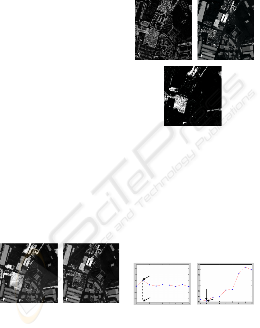
. Figure 1 shows the first-pulse and the
last-pulse LIDAR range image from the city of
Rheine in Germany. The impact of the Vegetation in
the first- and last- pulse images can be easily
recognized by comparing the two images of this
figure.
First pulse range Last pulse range
Figure 1: LIDAR dataset.
The first step in every clustering process is to
extract the feature image bands. The features of
theses feature bands should carry useful textural or
surface related information to differentiate between
regions related to the surface.
Relief range first Top-Hat range last
NDVI range
Figure 2: Three applied Feature.
Several features have been proposed for
clustering of range data. Axelsson (1999) employs
the second derivatives to find textural variations and
Maas (1999) utilizes a feature vector including the
original height data, the Laplace operator, maximum
slope measures and others in order to classify the
data. In our work, three types of features are taken
into account. These features are: NDDI ratio,
Morphological Opening and relief of range
information of LIDAR data. Figure 2 shows the
output of three mentioned features on LIDAR data
set.
To assess the validity of clustering algorithm we
experimented the algorithm for n
c
= 1 to n
c
= 10.
Using Davies-Bouldin (DB) and Hubert indices,
three clusters are optimum according to input data.
Plot of the indices
versus n
c
is depicted in Figure 3.
Hubert Index DB Index
Figure 3: Optimum Clusters.
Figure 4 shows outputs of the K-Mean, FCM and
SOM algorithms for the situation of optimum cluster
number (i.e. 3).
Maximum Hubert Index
Optimum Cluster
Minimum DB Index
Optimum Cluster
(
11
)
VISAPP 2006 - IMAGE UNDERSTANDING
152
K-Means
SOM FCM
Figure 4: The situation of optimum cluster number.
4 ANALYSIS OF CLUSTERING
RESULTS
After performing clustering algorithms (K-Means,
FCM and SOM), it is necessary to assess their
accuracies. In this context, the term accuracy means
the level of agreement between labels assigned by
the clustering algorithm and class allocation based
on truth data. To generate an appropriate truth data,
we used aerial image of the scene and first-pulse
range of LIDAR data. Using these data we produced
the ortho-image. Then, Buildings and vegetation
have been digitized, manually. Figure 5 shows the
truth data.
The method used in this paper to assess the
accuracy of clustering results is based on analysis of
the confusion matrix. The most common tool for the
clustering accuracy assessment is in term of a
confusion matrix. The columns in a confusion
matrix represent truth data, while rows represent the
labels assigned by the clustering algorithm. The
confusion matrix of K-Means, FCM and SOM
results, are presented in Table 1, respectively.
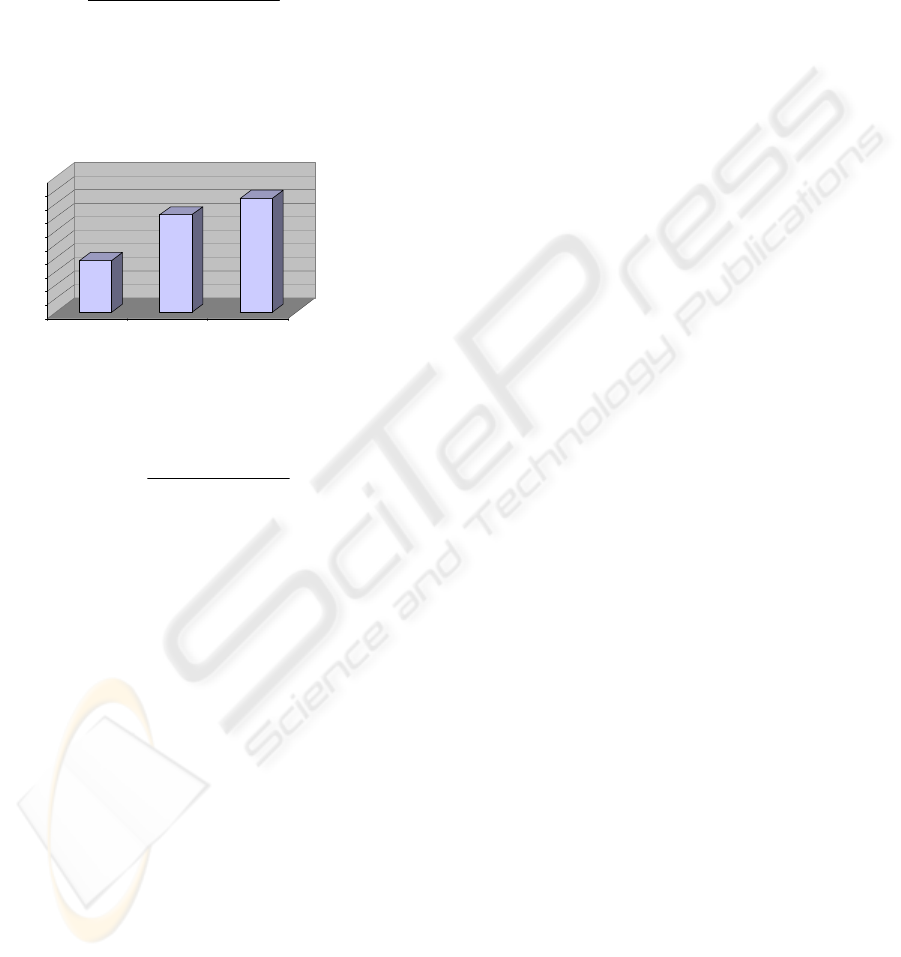
Several indices of clustering accuracy can be
derived from the confusion matrix. One of these
indices is "overall accuracy", which is obtained by
dividing the sum of main diagonal entries of the
confusion matrix by the total number of patterns.
Figure 6 shows the "overall accuracy" of K-Means,
FCM and SOM.
Man-made objects Vegetation
Truth Data
Figure 5: The truth data.
Table 1: Confusion matrix of K-Means, FCM and SOM.
Truth Data
Buildings Vegetation Bare-Land Sum
Buildings 64338 1551 338 66227
Vegetation 3561 58692 5930 68183
Bare-Land 54341 10509 290740 355590
K-Means
Sum 122240 70752 297008 490000
Buildings Vegetation Bare-Land Sum
Buildings 108835 4292 1697 114824
Vegetation 921 49488 517 50926
Bare-Land 12484 16972 294794 324250
FCM
Sum 122240 70752 297008 490000
Buildings Vegetation Bare-Land Sum
Buildings 116002 591 4666 121259
Vegetation 2224 63953 3344 69521
Bare-Land 4014 6208 288998 299220
SOM
Sum 122240 70752 297008 490000
The accuracy measurements shown above,
namely, the overall accuracy and producer's
accuracy, though quite simple to use, are based on
either the principal diagonal or columns of confusion
matrix only, which does not use the information
from the whole confusion matrix. A multivariate
Figure 6: Overall accuracy of K-Means, FCM and SOM.
84%
92%
96%
50%
55%
60%
65%
70%
75%
80%
85%
90%
95%
100%
K-Means FCM SOM
84%
92%
96%
EVALUATING THE POTENTIAL OF CLUSTERING TECHNIQUES FOR 3D OBJECT EXTRACTION FROM LIDAR
DATA
153
index called the kappa coefficient (Cohen, 1960) has
found favour. The kappa coefficient is defined as
Eq. (12) where k is number of clusters,
+i
M
and
i
M
+
are the marginal totals of row i and column i,
respectively and N is the total number of patterns.
()
()
∑
∑∑
=
++
==
++
⋅−
⋅−⋅
=
k
i
ii
k
i
k
i
iiii
MMN
MMMN
1
2
11
,
κ
(12)
Figure 7 shows the "kappa coefficient" of K-
Means, FCM and SOM.
The value of kappa for each cluster can be
derived as follows:
iii
iiii
i
MMMN
MMMN
+++
++
⋅−⋅
⋅
−
⋅
=
,
κ
(13)
5 CONCLUSION
Airborne laserscanning is being used for an
increasing number of mapping and GIS data
acquisition tasks. Besides the original purpose of
digital terrain model generation, new applications
arise in the automatic detection and modeling of
objects such as buildings or vegetation for the
generation of 3-D city models. A crucial prerequisite
for the automatic extraction of objects on the Earth's
surface from LIDAR height data is the clustering of
datasets. Besides the height itself, height texture
defined by local variations of the height is a
significant feature of objects to be recognized.
We have presented the results of applying three
different clustering techniques on LIDAR data for
3D object extraction. Using these methods we have
been able to filter non-terrain 3D objects such as
buildings and trees while keeping terrain points for
quality digital terrain modelling.
However, as it appear from obtained results of
applying different clustering methods on LIDAR
data; the SOM has the most reliable potential for
extraction of 3D objects like building and trees from
bare terrain.
REFERENCES
Axelsson, P., 1999. Processing of laser scanner data –
algorithms and applications. ISPRS Journal of
Photogrammetry and Remote Sensing, 54(2-3): 138-
147.
Cohen, J. 1960, "A coefficient of agreement for nominal
scales", "Educational and Psychological
Measurement", Vol. 20(1): pp. 37-46
Davies, D.L. and Bouldin, D.W. (1979). "A Cluster
Separation Measure." IEEE Transactions on Pattern
Analysis and Machine Intelligence, 1(2), 224–227.
Haala,N and Brenner, "Extraction of buildings and trees
in urban environments", ISPRS Journal of
Photogrammetry & Remote Sensing V 54(2-3), 130-
137 (1999).
Halkidi, M., Batistakis, I.and Vazirgiannis, M. (2001).
"On Clustering Validation Techniques", Journal of
Intelligent Information Systems, 17:2/3, 107–145
Hubert, L.J. Arabie, P., 1985, "Comparing
partitions",
Journal of Classification, Vol. 2, pp. 193-218.
Kohonen, T., 1989, "Self-Organization and Associative
Memory", Springer-Verlag.
Maas, H.G., 1999. The potential of height texture
measures for the segmentation of airborne
laserscanner data.
Mass, H. Vosselman, G. (2001), "Two algorithms for
extracting building models from raw laser" OEEPE
Workshop on Airborne Laserscanning and
Interferometric SAR for Detailed Digital Elevation
Models, Stockholm, Official Publication OEEPE
no.40,2001, 62-72
Roggero, M., 2002. "Object segmentation with region
growing and principal component analysis",
International Archives of Photogrammetry and
Remote Sensing, Vol. 34, Part 3A, Graz, Austria
Rottensteiner, F., Briese, Ch., 2002. "A new method for
building extraction in urban areas from high-resolution
LIDAR data", International Archives of
Photogrammetry and Remote Sensing, Vol. 34, Part
3A, Graz, Austria
Sithole, George, Vosselman, George,2003, "Comparison
of Filtering Algorithm"Proceedings of the Fourth
International Airborne Remote Sensing Conference,
Ottawa, Canada. pp. 154-161.
TopScan, 2004. Airborne LIDAR Mapping Systems.
http://www.topscan.de/en/luft/messsyst.html (accessed
10 Feb. 2004)
69%
86%
92%
50%
55%
60%
65%
70%
75%
80%
85%
90%
95%
100%
K-Means FCM SOM
69%
86%
92%
Fi
g
ure 7: Ka
pp
a coefficient of
K
-Means
,
FCM and SOM.
VISAPP 2006 - IMAGE UNDERSTANDING
154
