
THE USE OF DYNAMICS IN GRAYLEVEL QUANTIZATION BY
MORPHOLOGICAL HISTOGRAM PROCESSING
Franklin C
´
esar Flores, Leonardo Bespalhuk Facci
Department of Informatics, State University of Maring
´
a
Av. Colombo, 5790 - Bloco 19 - Zona 07, Zip Code 87020-900 - Maring
´
a - PR - BRAZIL
Roberto de Alencar Lotufo
School of Electrical and Computer Engineering, State University of Campinas
Av. Albert Einstein, 400 - PO Box 6101, Zip Code: 13083-970 - Campinas - SP - BRAZIL
Keywords:
Morphological processing, histogram classification, dynamics, watershed.
Abstract:
In a previous paper, it was proposed a method applied to image simplification in terms of graylevel and flat
zone reduction, by histogram classification via morphological processing. It this method, it is possible to
reduce the number of graylevels of an image to n graylevels by selecting n regional maxima in the processed
histogram and discarding the remaining ones, in other to classify the histogram via application of watershed
operator. In the previous paper, it was proposed the choice of the n highest regional maxima. By far, it is not
the best criterion to choose the regional maxima and other criteria had been were tested in order to obtain a
better histogram classification. In this paper we propose the selection of the regional maxima via application
of dynamics, a measurement of contrast usually applied to find markers to morphological segmentation.
1 INTRODUCTION
Color quantization is a very important research field
in digital image processing and computer graphics,
and among its contributions, it may be found sev-
eral techniques applied to simplification of images by
color reduction (Gonzalez and Woods, 1992; Heck-
bert, 1982; Soille, 1996). The importance of image
simplification by color reduction is clear when deal-
ing with problems of image display and image com-
pression (Gomes and Velho, 1994).
The application of color reduction techniques may
also provide the reduction of flat zones (connected re-
gions of pixels with constant color) in the image, such
a connected filter (Crespo et al., 1997; Salembier and
Serra, 1995; Heijmans, 1999; Meyer, 1998). The re-
duction of flat zones does not introduct borders in the
image, but, by supressing some borders, two of more
flat zones may be joined in one.
Flat zone reduction have a great number of appli-
cations. They can be, for example, applied to im-
age compression and image segmentation (Meyer and
Beucher, 1990; Beucher and Meyer, 1992). They are
also applied to reduce the statistics of the image, in
order to simplify the number of attributes used in pat-
tern recognition techniques (Hirata Jr. et al., 1999;
Flores et al., 2000; F. C. Flores and Zuben, 2002).
One simple way to reduce graylevels in an image
is the classical thresholding. Given a thresholding
value, the graylevels are classified by setting the pixel
value to white (maximum graylevel) if its graylevel is
higher than the thresholding value, or to black (min-
imum graylevel), otherwise. The classical threshold-
ing can be extended by applying a set of n threshold-
ing values, in order to reduce the number of graylevels
of an image to n +1graylevels: if a graylevel value
belongs to an interval given by a pair of thresholding
values, it should be replaced by the graylevel assigned
to that interval.
In a previous paper (Flores and Lotufo, 2001), it
was proposed a method which gives not only an im-
age simplification in terms of graylevel reduction but
also in terms of flat zone reduction. The proposed
method is given by application of a set of morpho-
logical operators to the image histogram. The main
motivation behind the project of this operator is that
each object in the image has a significative graylevel
distribution. So, to simplify an object in the image,
that is enough to classify its corresponding distribu-
tion in the histogram.
In that paper it was also proposed a method to re-
duce an image to n graylevels. It consists in to choose
the n highest regional maxima in the processed his-
togram and to filter the other peaks. The chosen max-
ima will provide the classification of the graylevels in
the histogram by application of watershed operator.
121
César Flores F., Bespalhuk Facci L. and de Alencar Lotufo R. (2006).
THE USE OF DYNAMICS IN GRAYLEVEL QUANTIZATION BY MORPHOLOGICAL HISTOGRAM PROCESSING.
In Proceedings of the First International Conference on Computer Vision Theory and Applications, pages 121-128
DOI: 10.5220/0001374501210128
Copyright
c
SciTePress

Note that, by far, it is not the best criterion to choose
the regional maxima and other criteria were tested in
order to obtain a better histogram classification.
In this paper we propose the application of dynam-
ics (Grimaud, 1992) to select the regional maxima in
order to achieve a better graylevel reduction. Dynam-
ics consists in a valuation of extrema of the image by a
measure of contrast that does not consider the size or
shape of valleys and peaks. It is usually applied to find
markers to morphological segmentationand achieve
hierarquical segmentation (Meyer, 1996).
Section 2 presents some preliminar definitions, and
section 3 presents the dynamics. Section 4 proposes
the technique to connected filtering by graylevel clas-
sification and a variation when it is possible to choose
the desired number of graylevels in the resulting im-
age. Section 5 presents some experimental results and
in the Section 6 we conclude this paper with a brief
discussion.
2 PRELIMINARY DEFINITIONS
Let E ⊂ Z×Z be a rectangular finite subset of points.
Let K =[0,k] be a totally ordered set. Denote by
Fun[E, K] the set of all functions f : E → K.An
image is one of these functions (called graylevel func-
tions). Particularly, if K =[0, 1], f is a binary im-
age. An image operator (operator, for simplicity) is
a mapping ψ : Fun[E, K] → Fun[E,K].
Let N(x) be the set containing the neighbourhood
(Hirata Jr., 1997; Flores, 2000) of x, x ∈ E.We
define a path (Hirata Jr., 1997) from x to y, x, y ∈
E as a sequence P (x, y)=(p
0
,p
1
, ..., p
n
) from E,
where p
0
= x, p
n
= y and ∀i ∈ [0,n − 1],p
i
∈
N(p
i+1
).
A connected subset of E is a subset X ⊂ E such
that, ∀x, y ∈ X, there is a path C entirely inside X.
Let f ∈ Fun[E,K].Aflat zone of f is a connected
subset X ⊂ E, such that f(x)=f(y), ∀x, y ∈ X.
Definition 1 The inf - reconstruction and sup - re-
construction operators are given, respectively, by,
∀f,g ∈ Fun[E, K],
ρ
B,g
(f)=δ
∞
B,g
(f)
ρ
∗
B,g
(f)=ε
∞
B,g
(f)
where B ⊂ E is the structuring element, n ∈ Z
+
and
δ
n
B,g
and ε
n
B,g
are, respectively, the n-conditional di-
lation and the n-conditional erosion operators (Serra,
1982; Heijmans, 1994). δ
∞
B,g
(f) (ε
∞
B,g
(f)) means
that the dilation (erosion) is applied till idempotency.
Let τ
i
: Fun[E, K] → Fun[E, [0, 1]], i ∈ K,bea
threshold function, where τ
i
(f)(x)=1,iff(x) ≥ i,
and τ
i
(f)(x)=0, otherwise.
Definition 2 Let f ∈ Fun[E,K]. A regional maxi-
mum is a flat zone Z such that f (z) >f(n), z ∈ Z,
n ∈ N,N ∈F
Z
, where F
Z
is a set of all flat
zones adjacent to Z (Flores, 2000). The regional
maxima of f is found by application of a operator
µ
max
B
c
: Fun[E,K] → Fun[E,[0, 1]], given by
µ
max
B
c
(f)=τ
1
(ρ
B
c
,(f+1)
(f)) ∨ τ
k
(f)
where B
c
⊂ E is the structuring element defining
connectivity.
A regional miminum is a flat zone Z such that
f(z) <f(n), z ∈ Z, n ∈ N,N ∈F
Z
, where F
Z
is a set of all flat zones adjacent to Z.
3 DYNAMICS
Dynamics (Grimaud, 1992; Meyer, 1996) is a trans-
formation which valuates the extrema of an image ac-
cording to a contrast measurement. One advantage of
application of dynamics is that, while some methods
such as morphological filters need a size parameter to
evaluate constrast, the dynamics measurement does
not take in account the size and the shape of image
structures.
The evaluation of constrast of a regional minimum
is a good way to provide markers to application of
watershed operator in the morphological segmenta-
tion framework: an hierarquical segmentation may be
achieved by selecting the regional minima which dy-
namics is higher than a thresholding value and assign-
ing markers to them (Meyer, 1996).
Definition 3 Let x, y ∈ E. The dynamics Dyn
f
of
a path P (x, y) on an image f ∈ Fun[E, K] is given
by,
Dyn
f
(P (x, y)) = { |f(x
i
)−f(x
j
)| : x
i
,x
j
∈ P (x, y)}
i.e., the dynamics of P (x, y) is given by the difference
in altitude between the points of highest and lowest
altitude of P(x,y).
Figure 1 shows the dynamics of a path between x
and y.
Grimaud (Grimaud, 1992) also defines the dynam-
ics between two points x, y ∈ E on an image f ∈
Fun[E, K] as
Dyn
f
(x, y)={
Dyn
f
(P (x, y)) : P (x, y), }
where P (x, y) is a path between x and y.How-
ever, it will not be applied here, since the histogram
is an 1-D signal and, therefore, there is only one
path between any two points from the domain of his-
togram function. So, it will be considered here that
Dyn
f
(x, y)=Dyn
f
(P (x, y)).
VISAPP 2006 - IMAGE FORMATION AND PROCESSING
122
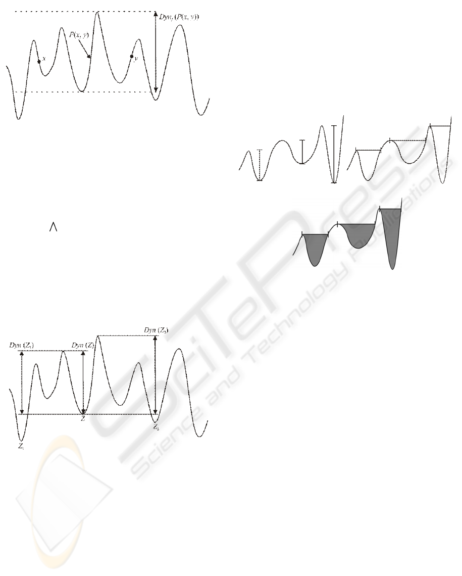
Figure 1: Dynamics of the Path Between x and y.
Definition 4 Let a(Z) ∈ K be the altitude of a re-
gional minimum Z in f . The dynamics of Z is given
by,
Dyn(Z)={ Dyn
f
(x, y),x ∈ Z, y ∈ M : a(M) <a(Z)}.
i.e., the dynamics of Z is given by the dynamics of the
path with the lowest dynamics that links Z to a point
y thats belongs to a catchment basin which regional
minimum has an altitude lower than Z.
Figure 2 illustrates the dynamics of a regional min-
ima Z.
Figure 2: Dynamics of a Regional Minimum.
Dynamics computation can be implemented by us-
ing tree of critical lakes (Meyer, 1996) or based on
flooding simulations algorithms (Grimaud, 1992).
Given the dynamics of a regional minimum Z,
some metrics can be used to evaluate such mini-
mum (da Silva, 2001):
1. depth of the catchment basin which the minimum is
contained (given by the dynamics of the minimum
itself) (Fig. 3 (a));
2. area of the catchment basin (Fig. 3 (b));
3. volume of the catchment basin (Fig. 3 (c));
Let us denote by Dyn
i
(f)(Z) the function that
computes to Z from f an value given by the metric
i ∈{1, 2, 3} introduced above. Dyn
i
(f)(Z) will be
used to evaluate the significant distributions in the his-
togram, as will be explained below.
Note that two catchment basin which have the same
depth may have different volume or area measure-
ments. Classification of regional minima in an image
can be achieved by application of such metrics.
(a) (b)
(c)
Figure 3: Dynamics: (a) Depth. (b) Area. (c) Volume.
4 THE PROPOSED TECHNIQUE
Let us introduce a new technique applied to con-
nected filtering. One characteristic of the proposed
filter is that, despite its connecting property, it does
not require a connectivity parameter (4-connect or 8-
connect) because all processing is done in the his-
togram of image.
As a consequence of such processing we have a
reduction in the graylevels appearing in the image.
In other words, the proposed filter is a mapping ψ :
Fun[E, K
1
] → Fun[E,K
2
], where |K
2
| < |K
1
|.
Let f ∈ Fun[E, K]. Let us consider the histogram
of the image as a function h
f
: K → Z
+
(Fig. 4). De-
spite the domain of h
f
, the morphological operators
used in the graylevel classification were applied to in
the same manner. In other words, we consider K as a
subset of E.
Let f ∈ Fun[E,K] and h
f
∈ Fun[K, Z
+
] its
histogram. Let max (h
f
) = max {h
f
(x):x ∈ K}.
Let κ : Fun[K, Z
+
] → Fun[K, Z
+
] be the mapping,
given by, ∀x ∈ K,
κ(h
f
)(x)=
h
f
(x),ifµ
max
B
(h
f
)(x)=1
0, otherwise
,
THE USE OF DYNAMICS IN GRAYLEVEL QUANTIZATION BY MORPHOLOGICAL HISTOGRAM PROCESSING
123
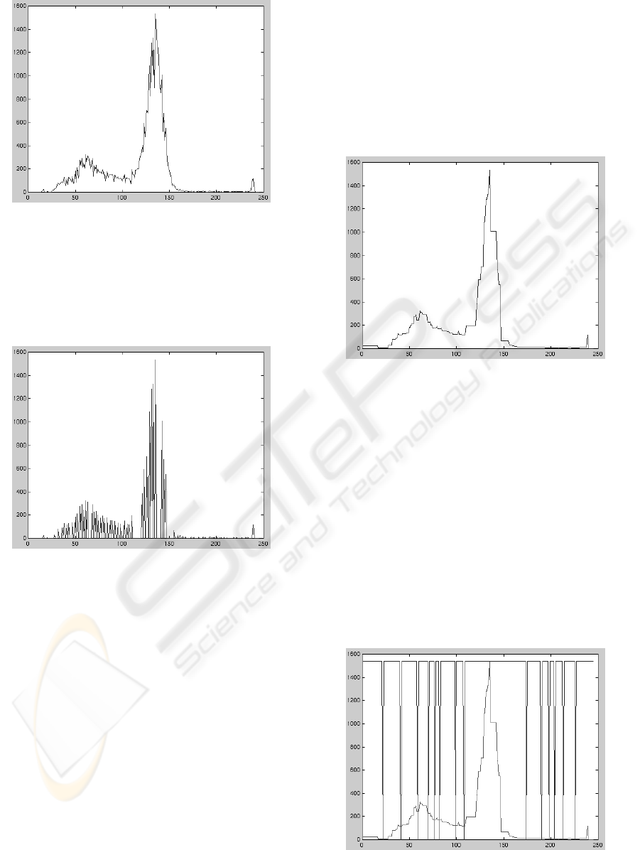
Figure 4: Histogram.
where B ⊂ K is the structuring element (Heijmans,
1994). The mapping κ gives a function with only the
regional maxima of h
f
. Figure 5 shows the regional
maxima of the histogram shown in Fig. 4.
Figure 5: Histogram regional maxima.
Let π : Fun[K, Z
+
] → Fun[K, Z
+
] be the map-
ping, given by, ∀x ∈ K,
π(h
f
)(x)=
max (h
f
),ifκ(h
f
)(x)=0
0, otherwise
.
Let η : Fun[K, Z
+
] → Fun[K, Z
+
] be the sup-
reconstruction of κ, denoted by,
η = ρ
∗
B,κ
(π),
where B ⊂ K is the structuring element.
If exists in κ(h
f
) a sequence of increasing regional
maxima followed by a sequence of decreasing re-
gional maxima, its regional maxima must compose
a curve whose regional maximum is the maximum
among them. The operator η is applied to the func-
tion κ(h
f
), in order to preserve the regional maxima
among the set of regional maxima of κ(h
f
) and con-
struct the curves with the remaining regional maxima
(Fig. 6).
The reason of the processing of the graylevel dis-
tributions in the histogram is that each object in the
image is represented by a significative graylevel dis-
tribution. The idea is to filter the histogram in order
to get new distributions where the objects are simpli-
fied and well represented. These new distributions are
used to get a meaningful classification of graylevels
by application of watershed operator introduced be-
low.
Figure 6: Reconstruction by application of η operator.
Let ω : Fun[K, Z
+
] → Fun[K, [0, 1]] be the
watershed operator (Beucher and Meyer, 1992; Vin-
cent and Soille, 1991). Let ν : Fun[K, Z
+
] →
Fun[K, Z
+
] be the negation operator.
Let λ : Fun[K, Z
+
] → Fun[K, Z
+
] be the map-
ping, given by, ∀x ∈ K,
λ(x)=
max (h
f
),ifω(ν(η))(x)=1
0, otherwise
.
The mapping λ gives a preliminary classification;
the graylevel classes are separeted but not labeled
(Fig. 7). The labeling of classes is given by the ap-
plication of next steps.
Figure 7: Pre-classification.
VISAPP 2006 - IMAGE FORMATION AND PROCESSING
124
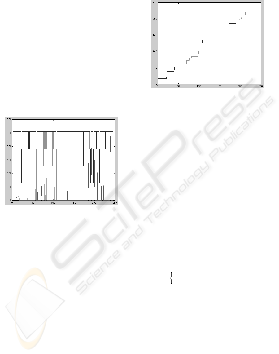
Let : K → Z
+
, such that (x)=x, ∀x ∈ K.
Let θ : Fun[K, Z
+
] → Fun[K, Z
+
] be the mapping,
given by, ∀x ∈ K,
θ(x)=
max (h
f
),ifµ
max
B
(η)(x)=1
0, otherwise
.
Let β : Fun[K, Z
+
] → Fun[K, Z
+
] be the mapping,
given by,
β = ∧ θ.
The mapping β gives a function where each point
of the regional maxima of η(·) is labeled by its cor-
responding graylevel. Its reconstruction conditioned
to λ(·) gives the labeling of all graylevel classes.
Figure 8 shows a composition of λ(·) (pre-classified
graylevels) and β(·) (the labeled peaks inside each
pre-class).
Figure 8: Function β assigning labels to each pre-class.
Let ζ : Fun[K, Z
+
] → Fun[K, K].
ζ = δ
B
(ρ
B,λ
(β)),
where B ⊂ K is the structuring element, and δ
B
(·) is
the dilation operator (Serra, 1982; Heijmans, 1994).
Let |K| be the number of distinct graylevels in K.
We can say that the mapping ζ is a graylevel classifi-
cator. Given the histogram h
f
, f ∈ Fun[E, K], the
classificator gives a new set of graylevels G, where
|G| < |K|. The processed histogram is used as a
look-up table in order to reduce the graylevels.
Definition 5 Let f ∈ Fun[E, K
1
], K
1
=[0,k
1
],
and h
f
∈ Fun[K
1
, Z
+
] the histogram of f . The
graylevel reducer by classification of regional max-
ima is a mapping ψ : Fun[E, K
1
] → Fun[E,K
2
],
where K
2
, |K
2
| < |K
1
|, is given by,
K
2
= ζ(h
f
).
Since there is a reduction in the number of graylevels
in the image, and it may causes the union of two or
more flat zones, without split any flat zone, it is a con-
nected operator. Figure 9 shows the graylevel classi-
fication provided by ζ, given the histogram shown in
Fig. 4.
Figure 9: Classified graylevels.
4.1 Reduction to n Graylevels by
Classification of Region Maxima
by Dynamics Metrics
When the operator ψ is applied to an image f , it re-
duces the graylevels appearing in f to the number of
regional maxima of η(·). However, it is possible to
reduce the graylevels to a smaller number, by adding
a parameter n which gives the number of graylevels
to appear in ψ(f ). In this section we will present a
way to select the n most significant regional maxima
of η(·) by application of dynamics.
We will denote by ψ
n
: Fun[E, K
1
] →
Fun[E, K
2
], |K
2
| < |K
1
|, |K
2
| = n, the operator
which performs the reduction of the graylevels in the
image to n graylevels.
Remember that the result of η operator is the orig-
inal histogram filtered in a way that the highest re-
gional maximum among a set of regiona maxima be-
longing to the same distribution is preserved. Let
D
i
: Fun[K, Z
+
] → Fun[K, Z
+
] be the function
given by,
D
i
(η)(x)=
Dyn
i
(ν(η))(Z):x ∈ Z,ifµ
max
B
(η)(x)=1
0, otherwise
,
where Z is one of the regional minima of the nega-
tion of η(·). I.e., if x belongs to a regional maximum
in η(·), D
i
(η)(x) will be equal to the dynamics (see
section 3) of the regional minimum where x is located
in the negation of η(·). i is the criterium chosen to
evaluate η(·): depth (1), area (2) or volume (3).
Let m be the number of regional maxima in η(·).
Let Q be the set defined by
Q = {q
i
∈ K : D
i
(η)(q
i
) > 0 and
D
i
(η)(q
i
) ≥ D
i
(η)(q
i+1
)),i=1, ··· ,m− 1}.
Let σ
n
: Fun[K, Z
+
] × n → Fun[K, Z
+
] be the
mapping, given by, ∀x ∈ K, ∀n ∈ Z
+
,
σ
n
(x)=
max (h
f
),ifx ∈ Q
0, otherwise
.
THE USE OF DYNAMICS IN GRAYLEVEL QUANTIZATION BY MORPHOLOGICAL HISTOGRAM PROCESSING
125
Let η
n
: Fun[K, Z
+
] × n → Fun[K, Z
+
] be the
mapping, given by, ∀x ∈ K, ∀n ∈ Z
+
,
η
n
= ν(ρ
∗
B,ν(η)
(σ
n
)).
By applying the operator η
n
, the n regional max-
ima of η(·) which have the highest dynamics are se-
lected. The function η
n
(·) contains just n regional
maxima and they are responsible for the classification
of n classes (given by application of watershed oper-
ator). The remaining peaks are removed.
The method proposed in section 4 can be now ex-
tended to reduce an image to n graylevels, by adding
the dynamics step introduced in this subsection to the
framework, before the application of the watershed
operator.
5 EXPERIMENTAL RESULTS
In this section, it will be presented two experimen-
tal results. In both presented experiments, it was ap-
plied the proposed method to graylevel reduction and
it were observed the simplification of the image in
terms of flat zones and the quality of the obtained
images. Four method were compared in both experi-
ments: the choice of n highest peaks selection (Flores
and Lotufo, 2001) and the three dynamics proposed
in this paper (depth, area and volume).
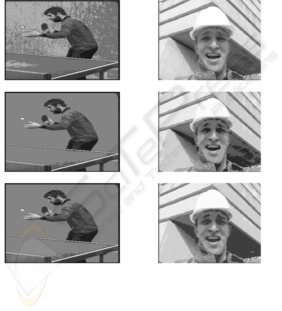
In the first experiment, it was aimed to simplify
the table tennis player (Fig. 10 (a)), an image with
66574 flat zones and 254 graylevels, to an image with
8 graylevels. It were applied the highest peaks method
and the four dynamics to reduce the image to the de-
sired amount of graylevels. Table 1 shows the amount
of graylevel reduction given by the application of each
criterion and Fig. 10 (b) and Fig. 11 (a-c) show their
respective results.
Note that the results given by the highest peaks and
the depth dynamics are close, both in flat zones reduc-
tion and the quality of image, and the depth dynamics
presented a slight better visual result. Area and vol-
ume dynamics provided the best results, both in the
simplification of the image and in the quality of the
resulting image.
The goal in the second experiment was to sim-
plify the foreman image (Fig. 12 (a)) to 10 graylevels.
This original image has 69301 flat zones and 252
graylevels. In this experiment, it was compared the
highest peaks to the volume dynamics. Figure 12 (b)
and (c), show, respectively the quantization provided
by application of both metrics. The highest peaks
provided a reduction to 6575 in the number of flat
zones and the volume dynamics provided a reduction
to 4757 flat zones. Note that the result provided by
the volume dynamics is also visually better: note that
the changes given by the dynamics metric is smoother
than the result given by the highest peaks criterion.
Table 1: Flat Zones Reduction.
Criterion Flat Zones
Original Image 66574
Highest Peaks 4375
Depth Dynamics 4595
Area Dynamics 2138
Volume Dynamics 1994
(a)
(b)
Figure 10: (a) Original Image (66574 Flat Zones). (b) High-
est Peaks (4375 Flat Zones).
6 CONCLUSION
This paper proposes an extension to a method applied
to graylevel quantization, proposed in a previous pa-
per (Flores and Lotufo, 2001). The method consists in
the classification of graylevels by application of mor-
phological operators to the histogram. Its result is a
new image with a fewer regions and a simplified col-
ormap, compared to the original image.
In the previous paper, it was proposed a way to
compute the reduction of graylevels to n levels, con-
sisting in the choice of the highest peaks and discard-
ing the remaining ones. The extension of this method
in given by the application of dynamics as a criterion
to the choice significant distributions in the histogram,
instead to choose the highest ones.
VISAPP 2006 - IMAGE FORMATION AND PROCESSING
126
(a)
(b)
(c)
Figure 11: (a) Depth Dynamics (4595 Flat Zones). (b) Area
Dynamics (2138 Flat Zones). (c) Volume Dynamics (1994
Flat Zones).
(a)
(b)
(c)
Figure 12: (a) Original Image (69301 Flat Zones). (b) High-
est Peaks (6575 Flat Zones) (c) Volume Dynamics (4757
Flat Zones).
THE USE OF DYNAMICS IN GRAYLEVEL QUANTIZATION BY MORPHOLOGICAL HISTOGRAM PROCESSING
127

Some experiments were done in order to compare
the highest peaks criterion to the dynamics metrics.
The goal in both experiments presented here was to
analyze the flat zone reduction provides by the met-
rics and the visual quality of the resulting images.
The two experiments showed better results provided
by the dynamics, especially the results given by the
volume dynamics.
Further work includes the investigation of alter-
native metrics to choose the distributions in the his-
togram and the extension of the method proposed in
this paper to color images.
REFERENCES
Beucher, S. and Meyer, F. (1992). Mathematical Morphol-
ogy in Image Processing, chapter 12. The Morpholog-
ical Approach to Segmentation: The Watershed Trans-
formation, pages 433–481. Marcel Dekker.
Crespo, J., Schafer, R. W., Serra, J., Gratind, C., and Meyer,
F. (1997). The flat zone approach: A general low-level
region merging segmentation method. Signal Process-
ing, 62(1):37–60.
da Silva, W. D. F. (2001). Marcadore M
´
ınimos Usando Wa-
tershed. PhD thesis, School of Electrical and Com-
puter Engineering, State University of Campinas.
F. C. Flores, S. M. P. and Zuben, F. J. V. (2002). Auto-
matic Design of W-Operators using LVQ: Application
to Morphological Image Segmentation. In IEEE Pro-
ceedings of International Joint Conference on Neural
Networks (IJCNN2002), pages 1930–1935, Honolulu,
Hawaii.
Flores, F. C. (2000). Segmentac¸
˜
ao de Seq
¨
u
ˆ
encias de Im-
agens por Morfologia Matem
´
atica. Dissertac¸
˜
ao de
Mestrado, Instituto de Matem
´
atica e Estat
´
ıstica - Uni-
versidade de S
˜
ao Paulo.
Flores, F. C., Hirata Jr., R., Barrera, J., Lotufo, R. A., and
Meyer, F. (2000). Morphological Operators for Seg-
mentation of Color Sequences. In IEEE Proceedings
of SIBGRAPI’2000, pages 300–307, Gramado, Brazil.
Flores, F. C. and Lotufo, R. A. (2001). Connected Filtering
by Graylevel Classification Through Morphological
Histogram Processing. In IEEE Proceedings of SIB-
GRAPI’2001, pages 120–127, Florianopolis, Brazil.
Gomes, J. and Velho, L. (1994). Computac¸
˜
ao Gr
´
afica :
Imagem. IMPA/SBM, Boston.
Gonzalez, R. C. and Woods, R. E. (1992). Digital Image
Processing. Addison-Wesley Publishing Company.
Grimaud, M. (1992). A New Measure of Contrast: the
Dynamics. In SPIE, editor, Image Algebra and Mor-
phological Image Processing III, volume 1769, pages
292–305.
Heckbert, P. (1982). Color Image Quantization for Frame
Buffer Display. Computer Graphics, pages 297–307.
Heijmans, H. J. A. M. (1994). Morphological Image Oper-
ators. Academic Press, Boston.
Heijmans, H. J. A. M. (1999). Introduction to Connected
Operators. In Dougherty, E. R. and Astola, J. T., ed-
itors, Nonlinear Filters for Image Processing, pages
207–235. SPIE–The International Society for Optical
Engineering,.
Hirata Jr., R. (1997). Segmentac¸
˜
ao de Imagens por Mor-
fologia Matem
´
atica. Dissertac¸
˜
ao de Mestrado, Insti-
tuto de Matem
´
atica e Estat
´
ıstica - USP.
Hirata Jr., R., Barrera, J., Flores, F. C., and Lotufo, R. A.
(1999). Automatic Design of Morphological Opera-
tors for Motion Segmentation. In Stolfi, J. and Tozzi,
C. L., editors, IEEE Proc. of Sibgrapi’99, pages 283–
292, Campinas, SP, Brazil.
Meyer, F. (1996). The Dynamics of Minima and Contours.
In P. Maragos, R. S. Butt, M., editor, ISMM 3rd. Com-
putational Imaging and Vision, pages 329–336.
Meyer, F. (1998). From Connected Operators to Levelings.
In Heijmans, H. and Roerdink, J., editors, Mathemat-
ical Morphology and its Applications to Image and
Signal Processing, Proc. ISMM’98, pages 191–198.
Kluwer Academic Publishers.
Meyer, F. and Beucher, S. (1990). Morphological Segmen-
tation. Journal of Visual Communication and Image
Representation, 1(1):21–46.
Salembier, P. and Serra, J. (1995). Flat Zones Filtering,
Connected Operators, and Filters by Reconstruction.
IEEE Transactions on Image Processing, 4(8):1153–
1160.
Serra, J. (1982). Image Analysis and Mathematical Mor-
phology. Academic Press.
Soille, P. (1996). Morphological Partitioning of Multiespec-
tral Images. Electronic Imaging, 5(3):252–265.
Vincent, L. and Soille, P. (1991). Watersheds in Digital
Spaces: An Efficient Algorithm Based on Immersion
Simulations. IEEE Transactions on Pattern Analysis
and Machine Intelligence, 13(6):583–598.
VISAPP 2006 - IMAGE FORMATION AND PROCESSING
128
