FINDING A COMMON QUADRATIC LYAPUNOV FUNCTION

USING CONICAL HULLS

Rianto Adhy Sasongko

Control and Power Group, Department of Electrical and Electronic Engineering, South Kensington Campus,

Imperial College London, London SW7 2AZ, United Kingdom

J. C. Allwright

Control and Power Group, Department of Electrical and Electronic Engineering & Centre for Process Systems Engineering,

South Kensington Campus, Imperial College London, London SW7 2AZ, United Kingdom

Keywords:

Positive semideﬁnite matrices, cone, conicall hull.

Abstract:

Consider a set of linear time-invariant continuous-time systems that is a convex hull with vertices formed by a

given set of systems. The problem of ﬁnding a common Lyapunov function v, speciﬁed in terms of a symmetric

positive deﬁnite matrix, for the convex hull of systems is tackled by searching for a symmetric positive deﬁnite

(PD) matrix P which causes dv/dt to be negative deﬁnite for each vertex system. The approach involves an

extension of an existing method for solving optimization problems for positive semideﬁnite (PSD) matrices

that is based on a representation of the cone of PSD matrices as a conical hull. The condition that the derivative

of the Lyapunov function for each vertex system is negative deﬁnite is converted naturally into the condition

that the matrix P belongs to the interior of the intersection of several conical hulls: one for each vertex system

to ensure dv/dt for it is negative deﬁnite. The determination of a P in the intersection is viewed as the

solution of a quadratic programme on the product space of the cones. Then the existing theory and algorithms

for conical hull problems are adapted to the solution of the quadratic programme. The numerical results

suggest that the proposed algorithm is faster than the projective method used in MATLAB for small problems.

Effort is being devoted to improve it for larger problem.

1 INTRODUCTION

For a family of dynamical linear continuous-time sys-

tems, obtaining a common Lyapunov function (CLF)

is desirable to ensure stability of all systems in the

convex hull of that set of systems or stability when the

system transits from one vertex of the convex hull to

another at any time (D.Liberzon, 2003). The impor-

tance of a common Lyapunov function for stabiliza-

tion of switched linear systems is discussed in (G.Xie,

2004), and the existence of a common Lyapunov

function for a set of asymptotically stable systems is

examined in (N.A.Bobylev, 2002) and (R.N.Shorten,

2003). An algorithm for obtaining a common Lya-

punov function, called the gradient method, is dis-

cussed in (D.Liberzon, 2003). A semideﬁnite pro-

gramming algorithm, called the projective method,

(A.Nemirovskii, 1994) can also be used for solving

such problems.

Here a new algorithm is proposed for ﬁnding a

common Lyapunov function; it is based on the con-

ical hull approach to the description of the set of sym-

metric positive semideﬁnite matrices, which will be

introduced later.

Let S denote the set of symmetric matrices from

n×n

. Let S

≥

be the set of positive semideﬁnite ma-

trices, and S

the subset of positive deﬁnite matrices,

from S.

For a set of N stable A

∈ R

n×n

, i = 1 : N ,

the function v(x) = x

P x is a common Lyapunov

function for the A

if P ∈ S satisﬁes

P + P A

< 0, ∀i ∈ [1 : N]

(1)

Solving (1) for such a P is a semideﬁnite program-

ming problem with the symmetric positive deﬁnite

matrix P as the variable.

In the following analysis, it will be convenient to

describe such P by vec(P), which is the vector con-

sisting of the entries of P in a certain order. In de-

tail, vec(P ) = [P (1, :)

; P (2, :)

; . . . ; P (n, :)

] ∈

(using MATLAB notation). Of course, P =

vec

−1

(p). Consequently condition (1) can be written

as:

p ∈ vec(S

) , ∀i ∈ [1 : N]

p ∈ vec(S

)

(2)

for

= −(A

⊗ I + I ⊗ A

) ∈ R

×n

(3)

113

Adhy Sasongko R. and C. Allwright J. (2006).

FINDING A COMMON QUADRATIC LYAPUNOV FUNCTION USING CONICAL HULLS.

In Proceedings of the Third International Conference on Informatics in Control, Automation and Robotics, pages 113-118

DOI: 10.5220/0001218001130118

 SciTePress

where ⊗ denotes the Kronecker product.

Since the A

are asymptotically stable, the M

are

non-singular. Therefore P = vec

−1

(p) solves (1) if

and only if

p ∈ M

−1

vec(S

), ∀i ∈ 1 : N

p ∈ vec(S

) ,

(4)

or if and only if p ∈ int(I), the interior of I, where I

is deﬁned by

I =

(

i=1

−1

vec(S

)

(5)

The solution p needs to be in the interior of I to guar-

antee the positive deﬁniteness of the corresponding

matrix P = vec

−1

(p).

Hence, there is a CLF of the form v(x) = x

P x if

and only if

I 6= ∅ (6)

and the problem of solving (1) is equivalent to that of

ﬁnding an interior point p of the intersection I, assum-

ing it has one.

The main contribution here is the development of

a computational method for ﬁnding a vector p in

interior(I), if there is one.

We have chosen to investigate the above formula-

tion since the other obvious formulation

min

∈S

≥

i=[0:N]

i=1

+kP

−βIk

(7)

leads to one additional conical hull being involved

(the purpose of β, a positive scalar, will become clear

near (22)).

The material is presented in the following way.

Some descriptions and properties of a conical hull

representation of the set of symmetric PSD matrices

is given in Section 2. An approach for ﬁnding a point

in the interior of I using the conical hull approach is

outlined in Section 3. More detail about the solution

of the CLF problem using conical hulls is also given

in this section. Numerical procedure and some results

for the CLF problem are given in Section 4. Finally,

the conclusions are given in Section 5.

2 A CONICAL HULL FOR PSD

MATRICES

2.1 Conical Hull Characterization

for Symmetric PSD Matrices

The background theory of symmetric matrices can

be found in various references, some of them are

(R.A.Horn, 1985) and (G.Strang, 1988). The de-

ﬁnitions of this section and the basic conical hull

theory and approach used throughout this paper

are from (J.C.Allwright, 1988) and (J.C.Allwright,

1989); most of the proofs can be found in these pa-

pers.

Symmetric PSD matrices are deﬁned uniquely by

their diagonal and upper triangle of elements, so

vec(S) = {vec(A) : A ∈ S} is a subset of a linear

subspace of R

that has dimension r = n(n + 1)/2.

An orthonormal basis for that subspace can easily be

found. For instance, for the case n = 3, suitable ba-

sis vectors are w

= e

, w

= (e

+ e

√

2, w

√

2, w

= e

, w

= (e

√

2, w

= e

where e

= [0 0 . . . 0 1 0 . . . 0]

with the 1 in row i.

The corresponding basis matrix is

W = [w

. . . w

] ∈ R

×r

(8)

and it is easy to check that W

W = I

, R[W

] =

and R[W] = vec(S).

Using this basis, vec(A) ∈ R

can be written in

terms of the vector vec(A) ∈ R

vec(A) = W vec(A) ∈ R

(9)

where

vec(A) = W

vec(A) ∈ R

. (10)

Since, generically, vec(A) contains no redundant

information regarding symmetric A, it can be thought

of as a minimal description of such an A.

Now any matrix A ∈ S

≥

can be written as A = M

for some M ∈ S. For example, if the spectral form of

A is written as V ΛV

with Λ = diag[λ

. . . λ

]

then such an M is V diag(

√

. . .

√

. Let-

ting B = M(kMk

)

−1

, where kMk

(

i,j=1

)

0.5

is the Frobenius norm, we see that

our general A can be written as A = αB

for α ∈

[0, ∞) and B ∈ U := {B ∈ S : kBk

= 1}. This

suggests, correctly, that S

≥

= cone{B

: B ∈ U}

where cone(X) := {αx : α ∈ [0, ∞), x ∈ X} is the

conical hull of X.

In fact, it will be more convenient to use

vec(S

≥

) = cone(Ω) (11)

where

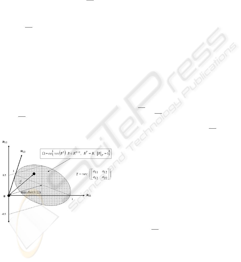
Ω = conv {Ψ} (12)

for

Ψ =



vec(B

) : B ∈ U



⊂ R

U =



B ∈ R

n×n

: B

= B , kBk

= 1



(13)

and it is obvious that the set vec(S

≥

) that contains

only the minimal description of every symmetric pos-

itive semideﬁnite matrix can be written as:

vec(S

≥

) = cone(W

Ω) (14)

ICINCO 2006 - INTELLIGENT CONTROL SYSTEMS AND OPTIMIZATION

114

2.2 Properties of our Conical Hull of

Symmetric PSD Matrices

Some deﬁnitions and properties of the conical hull

of PSD matrices are presented in this section; this

will be needed for the development of the algorithm.

Recall that vec(S

≥

) = cone(Ω) and vec(S

≥

) =

cone(W

Ω) for Ω of (12). Since the set S

symmetric positive deﬁnite matrices is the interior of

the set S

≥

vec(S

) = int(cone(W

Ω)) (15)

It follows from the deﬁnition (12) that Ω is a non-

empty, convex, and compact set, and (not so obvi-

ously) that:

min kxk

= n

−1/2

x ∈ Ω

(16)

A consequence of this fact is that:

min kxk

= σ

min

(L)n

−1/2

x ∈ LW

Ω

(17)

for all L ∈ R

r×r

, where σ

min

(L) is the minimum

singular value of L.

It is interesting that Ω is a subset of an afﬁne subset

of R

, which is actually the intersection of an afﬁne

set and (vec(S

≥

), which is a cone. Hence, somewhat

surprisingly, Ω is a ’ﬂat’ set. This is illustrated in the

following ﬁgure:

Figure 1: Depiction of Ω.

For the determination of feasible descent directions

later, it will be important to be able to solve easily, for

any vector ¯g ∈ R

, the optimization problem:

min ¯g

γ ∈ LW

Ω

(18)

It turns out that a minimizer ˆγ can be found easily as

ˆγ = LW

vec(νν

) (19)

where ν is a normalized eigenvector corresponding to

the minimum eigenvalue of Z, with Z deﬁned as:

Z = [vec

−1

(¯g) + vec

−1

]/2 ∈ R

n×n

(20)

for

¯g = W L

g (21)

3 OPTIMIZATION ON CONICAL

HULLS

Conceptually the CLF problem is that of ﬁnding a

¯z ∈ int(

) where the K

are the convex sets

cone(W

Ω). The approach will be to ﬁrst ﬁnd

a point in the intersection

and then, if it is not

in the interior, to perturb it into the interior (if there is

one).

The basic idea for ﬁnding a point in

is to

ﬁnd a ¯z

in each K

such that the distance between

all ¯z

is minimized. Then, if the minimal distance is

zero, we have found a point

¯z which is in the inter-

section

. Obviously the origin is not in the inte-

rior of the intersection, so to encourage the optimiza-

tion algorithm to ﬁnd a non-zero point, a penalty term

k¯z

− vec(βI)k

, with positive real β, is added to the

cost to attract vec

−1

(¯z) towards the positive deﬁnite

matrix βI. Hence the problem is

min

¯z

∈K

i=[1:N]

i,j∈[1:N]

i6=j

k¯z

− ¯z

+ k¯z

− vec(βI)k

(22)

which is a convex problem. Next a cone is constructed

as:

K = {K

× K

× . . . × K

} (23)

Then the optimization problem (22) can be reformu-

lated as :

min v(¯z)

¯z ∈ K

(24)

where,

v(¯z) = ¯z

Q¯z +

F ¯z

Q =

i,j=1, i6=j

F = −2

−

(25)

Here

β = vec(βI), ¯z = (¯z

, . . . , ¯z

)

with each

¯z

∈ K

, and the matrix

selects ¯z

from ¯z, in that

¯z

¯z.

The set K itself is a convex cone, so the algorithm

of (J.C.Allwright, 1988) for ﬁnding the closest point

in cone(Γ) to a point d , i.e. for solving

min kd − xk

x ∈ cone(Γ)

(26)

can be adapted to solve the optimization problem

above because kd −xk

= kdk

−2d

x + kxk

and

FINDING A COMMON QUADRATIC LYAPUNOV FUNCTION USING CONICAL HULLS

115

this has the same form as the cost of (22).

To proceed further, the notion of a truncated cone

is needed . The bounded subset cone

(Γ) =

{αx : x ∈ Γ, α ∈ [0, 1]} will be called the trun-

cation of the complete conical hull cone(Γ) =

{αx : x ∈ Γ, α ∈ [0, ∞]}. Then the corresponding

truncated cone K

is deﬁned by

= cone

(η

Ω) × cone

(η

Ω)×

. . . × cone

(η

Ω)

(27)

It turns out that it is easy to compute a positive real

η such that the unknown optimal solution of (22) lies

in the bounded set K

. This yields the optimization

problem

min v(¯z)

¯z ∈ K

(28)

An algorithm for solving this problem is discussed

next.

3.1 Finding Supporting Hyperplanes

The concepts and algorithm of (J.C.Allwright, 1988)

can now be applied to solve the optimization prob-

lem of (28). At each iteration, it ﬁrst calculating the

gradient ¯g

= 2¯z

Q − 2

(

) of the quadratic

cost v(¯z) . A linearisation about ¯z

of v(¯z) is then

provided by v(¯z

) + ¯g

(¯z − ¯z

). The next step is to

minimize this linearisation with respect to ¯z from K

by solving the problem:

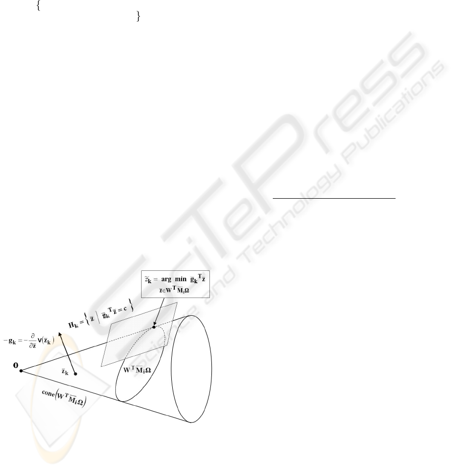
Figure 2: Linear minimization over cone.

min ¯g

(¯z − ¯z

)

¯z ∈ K

(29)

For suppose an optimal solution for this problem is

called ˜z

. Then ˜z

− ¯z

is a feasible descent direc-

tion from ¯z

and therefore can be used to decrease the

value of the cost fuction v(¯z). It can be seen that the

minimizer will be either in the set ηW

Ω or at the

origin i.e. at the vertex of the cone. An interpretation

of this optimization is that it is ﬁnding the supporting

hyperplane for the set K

that has normal ¯g

. Owing

to the structure of optimization problem (29), this lin-

ear programming problem can be decomposed into N

separate minimization problems

min ¯g

¯z

¯z ∈ K

i ∈ [1 : N]

(30)

where the gradients ¯g

are from the partitioning of

the gradient vector ¯g

¯g

. . . ¯g

According to (18-21), minimizing ¯g

(z) over the set

= cone

(η

Ω) will give the following

minimizer:

˜z

= η

vec(ν

) (31)

where η

is truncation factor for appropriate set and

is a normalized eigenvector corresponding to the

minimum eigenvalue of Z

, λ

min

], which is de-

ﬁned as:

(vec

−1

(

)) + (vec

−1

(

)

∈ R

n×n

(32)

with,

= W [¯g

W ]

(33)

Hence the contact point between set K

and support-

ing hyperplane H



¯z



¯g

¯z = C



is the vector

˜z



˜z

. . . ˜z



3.2 Quadratic Minimization Over a

Polytope

One way to determine a point ¯z

k+1

giving

v(¯z

k+1

) < v(¯z

) would be to minimize v(¯z) on

the set {¯z

+ ω(˜z

− ¯z

) : ω ∈ [0, 1]}. This involves

optimization with respect to the scalar ω and is

therefore relatively easy to carry out. This set is a

subset of K

so optimization on it can be regarded as

optimization of v(¯z) on an approximation to K

. Ob-

viously using a larger approximating set would tend

to give a greater reduction in v(¯z). Such a set can be

obtained as the convex hull of {0, ˜z

, ¯z

k−1

, ¯z

, . . .}.

Then ¯z

k+1

is chosen as the point in this convex hull

that minimizes v(¯z). A way to do this optimization

on the polytope is outlined next.

Having the contact points available, an approxi-

mation to the set K

is given by the convex hull of

the contact points (29) and the optimal points of (28)

from previous iterations. Then the minimizer of (28),

¯z, can be calculated by solving a quadratic problem

ICINCO 2006 - INTELLIGENT CONTROL SYSTEMS AND OPTIMIZATION

116

over this convex hull, as follows:

Theorem 3.1 : Let

¯z

k−N

¯z

k−N

, . . . ,

¯z

k−1

be the

set of minimizers of the quadratic function v(¯z) over

the convex hull deﬁned at iterations (k − N

), (k −

+ 1), . . . , (k − 1), and let ˜z

k−1

be the minimizer

of ¯g

k−1

(¯z − ¯z

k−1

) over K

at iteration (k −1). Then

¯z

) ≤ v(˜z

k−1

) ≤ v(

¯z

k−1

) (34)

where,

¯z

= arg min v(¯z)

¯z∈co

{

¯z

k−N

¯z

k−N

,...,

¯z

k−1

,˜z

k−1

}

(35)

Here co



¯v

, ¯v

, . . . , ¯v



represents the convex hull

of the vectors ¯v

, ¯v

, . . . , ¯v

and N

denotes the

number of vectors used for the convex hull. The inte-

ger k denotes the iteration number.

To solve optimization problem (35), we ﬁrst repre-

sent the variables ¯z

of each set K

as a convex com-

bination of ¯v

, ¯v

, . . . , ¯v

, i.e.

¯z

j=1

¯v

for

j=1

= 1, µ

≥ 0

(36)

for all i ∈ [1 : N] with each v

∈ R

(r×1)

Using this in (35) transforms the problem into the

quadratic programme in ˜µ

min

˜µ∈R

×N)×1

˜µ

QV˜µ +

F V˜µ

subject to G

˜µ =



((N

×N)×1)



˜µ ≥ 0

(37)

where

V =







(r×N

)

. . .

(r×N

)

(r×N

)

. . .

(r×N

)

(r×N

)

(r×N

)

. . .







(38)







(1×N

)

(1×N

)

. . .

(1×N

)

(1×N

)

(1×N

)

. . .

(1×N

)

(1×N

)

. . .

(1×N

)







(39)

with

¯v

. . . ¯v

˜µ = [¯µ

¯µ

. . . ¯µ

]

¯µ

= [µ

. . . µ

]

; i = 1, . . . , N.

(40)

Here

(p×q)

is a p ×q zero matrix and

p×q

is a p ×q

matrix with all its entries equal to 1.

The optimal solution,

¯z, of the original problem

(35) can then be calculated from the solution

˜µ of the

transformed problem (37) using

¯z = [V

]

˜µ (41)

where V

is as deﬁned in (38) with its entries formed

from the vectors specifying the convex hull deﬁned in

the last iteration.

The convergence of the sequence ¯z

to an optimizer

for optimization problem (22) can be proved in much

the same way that convergence for a similar optimiza-

tion problem was proved in (J.C.Allwright, 1988).

3.3 Correction Using Gradient

It may happen that the solution

P = vec

−1

¯z

)

from (41) above lies on one or more of the boundaries

of the cones K

, in which case the solution will not

satisfy at least one of the positive-deﬁniteness con-

straints. Even if the all the positive-deﬁniteness con-

straints are satisﬁed, it might be desired to have a ma-

trix that is not so close to the boundary in that the

smallest eigenvalue of −(A

P +P A

) is undesirably

small. In this case, a correction using the gradients of

the constraints can be incorporated into the algorithm.

This enables a small update δP to be applied to the so-

lution

P to give the modiﬁed solution

P + δP where

the correction can be obtained by ﬁnding a δ

P that

makes the following inequalities hold for all j:

l,m∈[1:n]

∂λ

(

M(i))

∂P

l,m

≤ 0, i ∈ I

−

l,m∈[1:n]

∂λ

(

M(i))

∂P

l,m

< 0, i ∈ I

l,m∈[1:n]

∂λ

(

M(i))

∂P

l,m

< 0, i ∈ I

(42)

Here (l, m) is the index of the elements of

P =

vec

−1

(

¯z), and

M(i) = A

P + P A

. I

−

, I

, and

denote the index of sets where the initial point

lies inside the corresponding set, on its boundary or

outside, respectively. It is obvious that for i ∈ I

−

i ∈ I

, and i ∈ I

, the value of

M(i) will be nega-

tive, zero, and positive respectively.

The gradient can obtained from:

∂λ

(

M(i))

∂P

l,m

= x

(43)

with x

is the eigenvector corresponding to the eigen-

value λ

(

M(i)). The δ

P will make the inequalities

in (42) hold, and it can be used for updating δP i.e.

we can set δP = ωδ

P by choosing an appropriate

scalar ω > 0, so that all constraints are satisﬁed by

the corrected solution.

4 NUMERICAL CALCULATION

4.1 The Algorithm

The algorithm then is implemented in numerical cal-

culation for solving our convex problem. The algo-

rithm is arranged as follows:

FINDING A COMMON QUADRATIC LYAPUNOV FUNCTION USING CONICAL HULLS

117

1. set k = 0, choose initial point ¯z

, error bound  >

0, number of vertices of the convex hull N

, and

calculate basis matrix W and

for all i

2. set ¯z = ¯z

3. calculate cost value v(¯z

) and the gradient ¯g

, then

ﬁnd the the contact point

¯z

between set K

and

hyperplane H

by solving ¯g

¯z (29)

4. for co {¯z

, ¯z

k−1

, . . . , ¯z

k−N

¯z

}, if k < (N

−

1) then set ¯z

k−1

, . . . , ¯z

k−N

= 0, form V and

, and calculate V

QV and

F V

5. solve the quadratic programming problem (37) to

get the minimizer

¯z

, and calculate v(

¯z

) and the

lower bound b

low

= v(¯z

) + ¯g

(

¯z

− ¯z

)

6. if v(

¯z

)−b

low

<  then stop, otherwise set ¯z

k+1

¯z

and k = k + 1 and go to step 2

7. perform correction procedure of section 3.3 if nec-

essary

4.2 Numerical Results

The algorithm has been tested for ﬁnding a com-

mon Lyapunov function for a various problems. The

results were compared with those of the projective

methods (A.Nemirovskii, 1994) available in the MAT-

LAB LMI toolbox. A common symmetric PD matrix

P was found after ﬁnite iterations using the conical

hulls, and the computing times for it are listed in 2nd

row of table 1. The 3rd row shows the processing time

for the correction procedure. The conical hull algo-

rithm and the MATLAB algorithm were executed 100

times to observe the consistency of the time calcula-

tions. Since the latest version of MATLAB exploits

the JIT-accelerator, converting the M-script to C/C++

code (MEX-ﬁle) would not have improved the execu-

tion time.

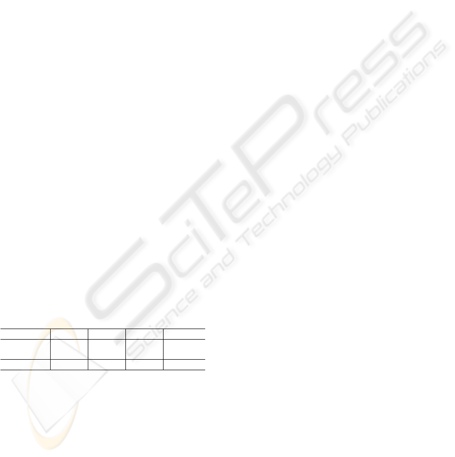
Table 1: Numerical Results - Processing time (seconds).

n = 10 N = 2 N = 4 N = 6 N = 10

C − Hull 0.003 0.0502 0.11 0.384

(corrct) 0.023 0.0411 0.0576 0.06

P rojM et 0.0633 0.0805 0.1063 0.2484

The results show that the conical hull algorithm

is faster for N = 2, 4. As the number of inequal-

ities increases, the conical hull algorithm becomes

slower, compared to the projective method. Since the

proposed method uses distance minimization between

points in all the cones, as the number of inequalities

rises, the number of variables will also rise signiﬁ-

cantly. Probably, the reason the conical hull algo-

rithm performs less well for bigger problem is that

the QP involved at each iteration becomes relatively

more costly to execute. To overcome this problem,

an efﬁcient way for managing the variables should be

explored. It should be noticed that the proposed algo-

rithm guarantees all the inequalities are satisﬁed ac-

curately.

5 CONCLUSIONS

A new algorithm has been presented, based on the ex-

isting conical hull theory, for solving the problem of

ﬁnding a common quadratic Lyapunov function for

a family of stable dynamical systems. The numeri-

cal results suggest that the algorithm is better than the

projective method for small problems. Further devel-

opments will be carried out to improve it for larger

problems and apply it to control studies.

ACKNOWLEDGEMENTS

The ﬁrst author would like to thank the Islamic De-

velopment Bank (IDB) who provides the fund that en-

ables him to undergo the project.

REFERENCES

A.Nemirovskii (1994). The projective method for solving

linear matrix inequalities. Proceedings of the Ameri-

can Control Conference, pages 840–844.

D.Liberzon (2003). Gradient algorithm for ﬁnding common

lyapunov functions. 42nd IEEE Conference on Deci-

sion and Control, pages 4782–4787.

G.Strang (1988). Linear algebra and its applications. Har-

court Brace Jovanovich, San Diego, 3 edition.

G.Xie (2004). Stability and stabilization of switched linear

systems with state delay: continuous-time case. 16th

Mathematical Theory of Networks and Systems Con-

ference.

J.C.Allwright (1988). Positive semideﬁnite matrices : Char-

acterization via conical hulls and least-squares solu-

tion of a matrix equation. SIAM journal of Control

and Optimization, 26:537–556.

J.C.Allwright (1989). On maximizing the minimum eigen-

value of a linear combination of symmetric matrices.

SIAM journal on Matrix Analysis and Applications,

10:347–382.

N.A.Bobylev, e. (2002). On the stability of families of dy-

namical systems. Differential Equations, 38(4):464–

470.

R.A.Horn (1985). Matrix Analysis. Cambridge University

Press.

R.N.Shorten (2003). On common quadratic lyapunov func-

tions for pairs of stable lti systems whose system ma-

trices are in companion form. IEEE Transactions on

Automatic Control, 48(4):618–621.

ICINCO 2006 - INTELLIGENT CONTROL SYSTEMS AND OPTIMIZATION

118