IMPROVED METHOD FOR HIGHLY ACCURATE INTEGRATION
OF TRACK MOTIONS
Michael Kleinkes, Werner Neddermeyer and Michael Schnell
University of Applied Science in Gelsenkirchen
Neidenburger Str. 43, 45897 Gelsenkirchen
Keywords:
Industrial robots, 7
th
axis, linear track, offline programming, motion control, flexible automation.
Abstract:
Modern Robotics today deals with increasing requirements on the flexible automation. One of this is the usage
of linear tracks or even called 7
th
axis to extend the robots workspace. The inaccuracies of the linear track
deteriorate the accuracy, which is in constrast to highly accurate robot systems needed for modern applications.
To enhance the accuracy of the system consisting of robot and linear track, an identification of the non-
linearities of the linear track is necessary. This article introduces an optimisation of a method for highly
accurate integration of track motions where the profile of the linear track is identified by single coordinate
systems along the track, combined by a cubic spline interpolation. Resulting there is a continous description
of the track profile, depending on the current position of the robot on the linear track.
1 INTRODUCTION
Modern industrial robot applications become more
and more complex. The increasing demand on flex-
ibility and automation effects the need of high preci-
sion robot systems. One part of this robot systems are
external linear tracks, even called 7
th
axis, on which
the robot can be linear moved to extend its workspace.
In most of the cases this extension of the workspace
via linear track deteriorates the accuracy of the sys-
tem robot and track in significant number about sev-
eral millimeters or more. This alarming fact is not
compatible to the demands on the flexible automation
at all and additionally is neglected by scientists and
robot manufacturers at well.
In (6) there is one method presented, which makes it
possible to identify the inaccuracies of the linear track
and correct offline robot programs. For this, the linear
track is measured at n positions where a correspond-
ing track coordinate system is calculated. The number
of positions on the linear track where the single track
coordinate systems are calculated - following called
sampling points - are determined by a frequency scan
of the linear track. To get a continous description of
the linear track these track systems are combined by
a cubic spline interpolation. By this it is possible to
get a correction frame for each arbitrary position on
the linear track. This paper sets up on the first arti-
Figure 1: Track coordinate systems.
cle about highly accurate integration of track motions
and presents optimisations in the fields of frequency
check and spline correction and fulfils parts of the fu-
ture prospects of this article.
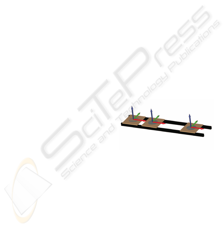
2 TRACK PROFILE FREQUENCY
CHECK
For the identification of the track motion one rigid
object is needed, which is to measure at different
positions on the linear track, by an 3D-coordinate
measurement device. Basing on the fact that the
rigid object is not deformed after moving from one
469
Kleinkes M., Neddermeyer W. and Schnell M. (2006).
IMPROVED METHOD FOR HIGHLY ACCURATE INTEGRATION OF TRACK MOTIONS.
In Proceedings of the Third International Conference on Informatics in Control, Automation and Robotics, pages 469-473
DOI: 10.5220/0001203504690473
Copyright
c
 SciTePress

position to the next position on the linear track, the
positional changings of some measurement points on
the rigid object are only caused by the linear track.
The very high reapeatability of modern industrial
robots makes it possible to use the robot as such a
rigid object. The inaccuracy in moving to one point
repeatedly is in most of the cases more then 10 times
less than the inaccuracies caused by the linear track.
In (7) there is an overview about the absolute and
repeat accuracy of the used robot.
One important step in the process of identifying
the linear track is the determination of the needed
number of sampling points on the track. This value
is depending on the maximum error which has to be
identified and varies with each individual linear track.
A special procedure developed before is here used
again and is in certain ways optimised. For this,
the robot is moved along the linear track with its
Tool-Center-Point (TCP) in one constant position.
During the robots movement it is measured by
the external measurement system in a continious
measurement mode. This creates measurement data
from a theoretical straight line movement disturbed
by the inaccuracies of the linear track on the one
hand, the robots own vibrations and the measurement
inaccuracies on the other hand.
So if we sperate the theoretical path from the mea-
surement results we get:
h
k
=
p
∆x
2
+ ∆y
2
+ ∆z
2
− s
k
(1)
with
s
k
= k · v · dt , k = 0, 1, . . . , N − 1 (2)
Taking this function h
k
we make the discrete fourier
transform on it and get the spectrum of the non-
linearities of the track. One special aspect not con-
sidered before is the spectral leakage effect of time
delimited functions. Considering the finite number of
measurement values taken in a finite time intervall,
the number of the discrete function values of h
k
is
N − 1 as can be seen in (1). In respect to this, there
is a convolution with the spectrum of the rectengular
function in the frequency domain.
So:
H(f
n
) =
Z
∞
−∞
h(s)e
−j2πf
n
s
ds ∗ G(rect
n
) (3)
and
G(rect
n
) = T
p
· si(πfT
p
) , T
p
=
1
f
n
(4)
This convolusion causes new spectral components
which are not included in the measured signal
whereby the original spectrum can not be analysed
properly. The solution for this problem is finding a
adequate window function, where the leakage effect
is lower, so that the important spectral components
can be detected properly.
The appropriate window function, a bartlett window
was found in some special analyses and after some
experiments in comparing different window functions
on the measurement values the discrete fourier trans-
form gets now an improved spectrum of the linear
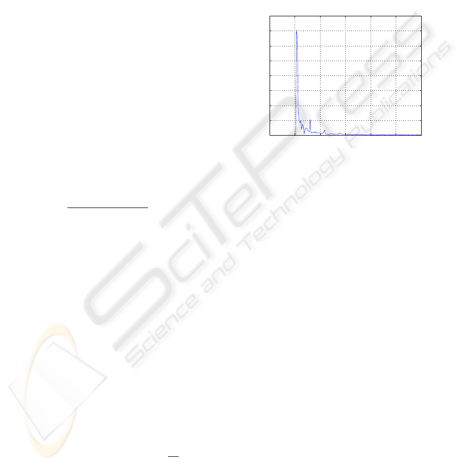
track scan depicted in figure 2:
−0.005 0 0.005 0.01 0.015 0.02 0.025
0
0.1
0.2
0.3
0.4
0.5
0.6
0.7
0.8
spectrum of h(t) with bartlett window
frequency [1/mm]
amplitude [mm]
Figure 2: Spectrum of the track scan.
Due to the windowing three different frequency peaks
can be seen clearly. The first peak with an amplitude
of 0.7 mm at a frequency of 0.0003/mm represents the
maximum error caused by the track which was mea-
sured and as you can see it is at the lowest frequency.
The other two peaks at 0.003/mm and 0.006/mm are
caused by the robots vibration and by the measure-
ment system.
To get the needed number of sampling points for an
identification of the linear track the new spectrum of
the windowed function is used, considering the sam-
pling theorem. With this new results the number of
sampling points can be reduced by 25%.
3 POSITIONING ERRORS DUE
TO SPLINE LINEARISATION
The benefit of the interpolation of the identified track
coordinate systems via cubic splines is a continous
description of the linear track in 6 dimensions
(x, y, z, α, β, γ). As already mentioned the single
track coordinate systems are identified in the sam-
pling positions depending on the frequency spectrum
after the continous track scan. So what we get after
calculating the track coordinate systems is:
T
R
i
W
= f
i
(α(l
i
), β(l
i
), γ(l
i
), t
x
(l
i
), t
y
(l
i
), t
z
(l
i
))
(5)
ICINCO 2006 - ROBOTICS AND AUTOMATION
470

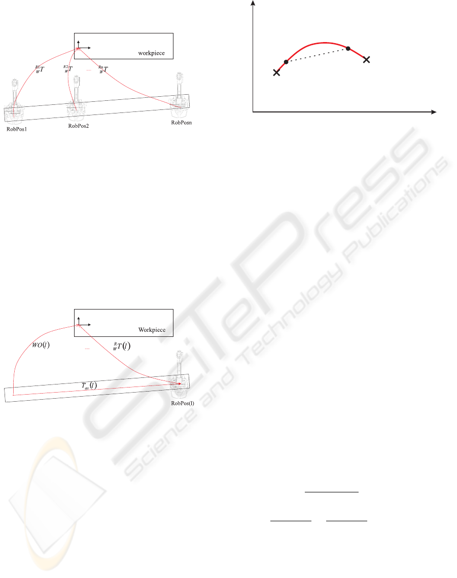
Figure 3: Track coordinate systems in sampling points.
This T
R
i
W
is depending on the sampling point position
i. Now we make use of the cubic spline interpolation
method and connect the discrete pairs of varieties
(α
i
, l
i
), (β
i
, l
i
), etc. with smooth and also smooth in
the first derivate functions, so that we can create track
coordinate systems on every arbitrary position on the
linear track.
T
R
W
(l) = f
i
(α(l), β(l), γ(l), t
x
(l), t
y
(l), t
z
(l)) (6)
Figure 4: Track coordinate systems arbitrary.
Using the continous description of the linear track
one robot programm can be modified and every
single position can be corrected considering its
corresponding linear track value. This method works
quite good for programs in which the robot moves
to static points. One crucial situation are linear
movements, because for this the robot uses two
programmed points and moves along the straight path
between these two points. The ability to correct the
first and the last point of this linear movement causes
that the robot moves at the start and end position
of its movement quite right, considering the errors
given through the linear track. But whats about all
the positions between the start and end point? Lets
make a small example:
The two positions p
1
and p
2
as shown in figure 5 are
S (x)
i
Lineartrackposition[mm]
Position[mm]
p
1
p
2
Figure 5: Programmed points between sampling positions.
programmed on a linear track position between two
sampling points. Between this two sampling points
there is the interpolation cubic spline function S
i
(x).
Assuming that the robot moves from the point p
1
to
the point p
2
it will calculate a straight line movement
using the new corrected positions for p
1
and p
2
. This
calculation will effect that during the movement no
correction can be processed because the splines are
not directly integrated into the positional control of
the robot. Mathematically the linearisation can be
described as follows:
Taking the general equation for cubic spline in
the range from one sampling position to the next:
S
i
(x) = a
i
+ b
i
(x − x
i
) + c
i
(x − x
i
)
2
+ d
i
(x − x
i
)
3
(7)
in the intervall I = [x
i
, x
i+1
]. To find one spline
function in the given interval there are four different
parameters to identify (a
i
...d
i
). Due to the side
conditions of the cubic spline interpolation there are
for each unknown spline four different equations to
find the four unknown parameters. As shown in (5) it
is possible to transform this set of equations to a set
of equation only depending on one parameter c
i
so
that:
d
i
=
1
3(x
i+1
− x
i
)
c
i−1
− c
i
(8)
b
i
=
y
i+1
− y
i
x
i+1
− x
i
−
x
i+1
− x
i
3
(c
i+1
+ 2c
i
) (9)
and
a
i
= y
i
(10)
with x
n
as x-coordinate in the sampling points and
therefore as linear track value at this positions and
y
n
as the corresponding y-coordinate of the single
dimension (x, y, z, α, β, γ). The remaining c
i
-values
IMPROVED METHOD FOR HIGHLY ACCURATE INTEGRATION OF TRACK MOTIONS
471

can be calculated through a linear equation using a
tridiagonal, symmetric and positive Matrix:
~c =
~
A
−1
· ~a (11)
with
~
A =



2(h
0
+ h
1
) h
1
0 0 0
h
1
2(h
1
+ h
2
) h
2
0 0
0 h
2
2(h
2
+ h
3
) h
3
0
0
.
.
.
.
.
.
.
.
.
0
0 0 0 h
n−2
2(h
n−2
+ h
n−1
)



(12)
using
h
i
= x
i+1
− x
i
(13)
and
~a =






3
y
2
−y
1
h
1
− 3
y
1
−y
0
h
0
− h
0
c
0
3
y
3
−y
2
h
2
− 3
y
2
−y
1
h
1
.
.
.
3
y
n
−y
n−1
h
n−1
− 3
y
n−1
−y
n−2
h
n−2
− h
n−1
c
n






(14)
Basing on this the prefactor d
1
of a spline between
two arbitrary points can be calculated:
d
1
=
6
15h
3
[(y
1
− y
0
) − 2(y
2
− y
1
) + (y
3
− y
2
)]
(15)
Special mathematical simulations have shown that
the greatest deviation from a straight line between
two points on the spline and the spline function itself
is when the cubic part and therefore the prefactor d
i
of the corresponding spline is zero. Basing on the
symmetry in (15) this is the case for y
2
= y
1
and
(y
1
− y
0
) − (y
3
− y
2
) = 0. Given this conditions the
maximal deviation is:
∆s = S
i

b
i
2c
i
+ x
i

− y
1
(16)
With practical meanings this is on a linear track with
an inaccuracy of 0,5 mm in the heigth of its two
rails an ∆s-value of 0.325mm. That means, that if it
would be possible to correct the robots position dur-
ing the movement, the postioning of the TCP would
be 0.325 mm better than without. Methods of correct-
ing the robots TCP-motion dynamically during the
movement were analysed and we expect to obtain ∆s-
values greater than 0.5mm.
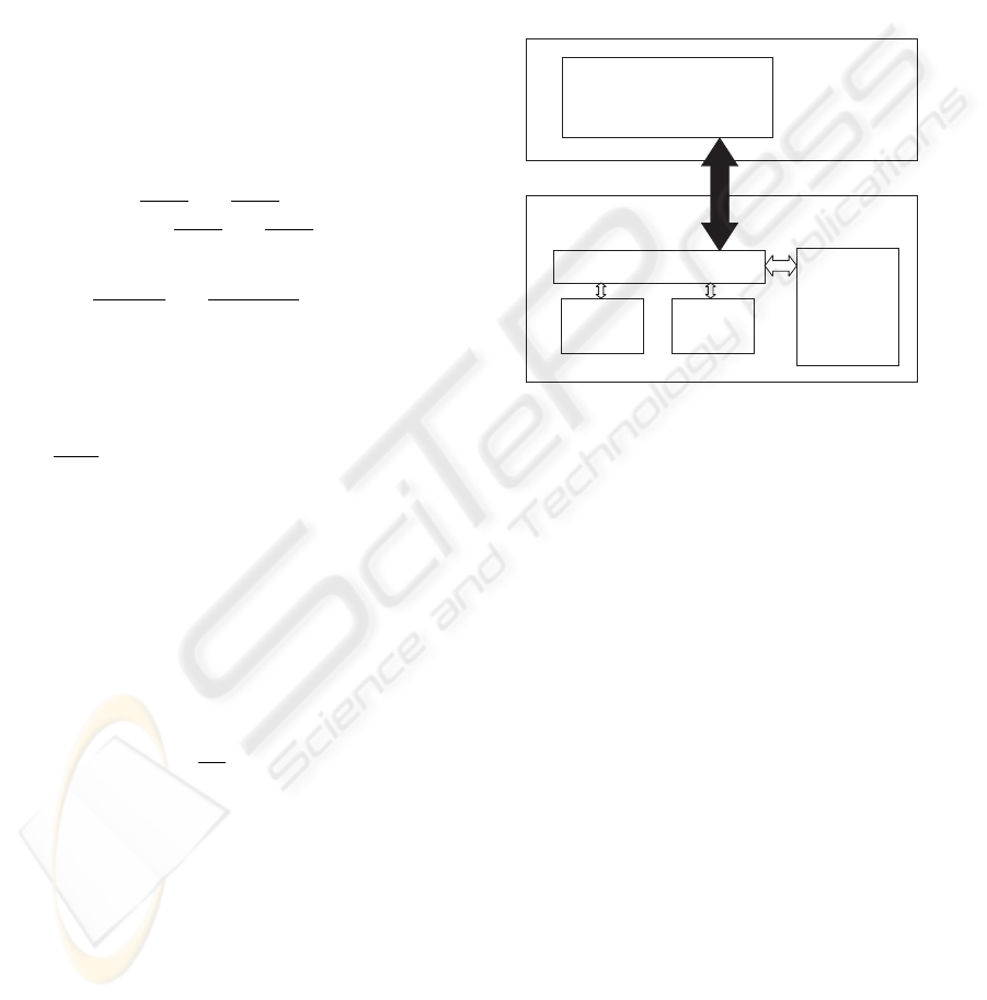
4 ROBOT INTERFACE
Due to a new robot interface it is possible to use an
uniform interface for variable sensor applications. For
this the used sensors are not connected to the robot
control via external interfaces but directly integrated
in the robots programming language. This is done
through a modular built program which is working on
the robot control an which is supporting special func-
tions for the user.
Realtimecore
Robot
Position
Control,
I/Os
Interfaceprogram
Sensors,
Drivers
Object
Libraries
Usercore
Robot
Programming
Language
Figure 6: Robot interface for dynamic correction.
Using this new robot interface it is possible to send
correction signals to the robot which are processed
exactly in the interpolation rate of the robot. This al-
lows to modify the TCP position with such a high time
rate that the spline correction can be nearly perfectly
used.
5 MEASUREMENT SYSTEM
The used measurement system for the needed mea-
surement tasks like continous scan of one track mo-
tion, determining the particular track coordinate sys-
tems or identifying of the robots accuracy is repre-
sented by a Leica Laser Tracker LTD800 (figure 7).
With this measurement device it is possible to do
touchless measurements of 3-dimensional points in a
range up to 80 meters. The measurement uncertainty
of a coordinate is given by 10µm + 5µm/m with a
possible maximum measurement rate of 3000 points
per second.
Using the world’s most accurate absolute distance
meter (25µmm within 40m) and two built-in preci-
sion encoders for horizontal and vertikal angle mea-
surements, it is a highly accurate measurement sys-
tem and common in measurement tasks for aircraft
and automobile industries.
ICINCO 2006 - ROBOTICS AND AUTOMATION
472

Figure 7: Leica LTD800 Laser Tracker.
6 CONCLUSION
The dynamic correction of the robot during its move-
ment is the basis for an optimal usage of the spline
interpolation. In the first step (6) there was only a cor-
rection of single points and as can be seen, this has an
disadvantage at controlled movements between two
points.
With the improved method for highly integration of
track motions this problem is solved and any move-
ment can be corrected. Even the offline correction
of robot programs is not needed anymore because the
robot gets the corrections in the interpolation cycle of
the motion control.
A future prospect will be the implementation of the
spline correction in the new interface modul and
therefore the correction of arbitrary movements.
REFERENCES
Bachman, G., Narici, L., Beckenstein, E. (2002). Fourier
and wavelet analysis. Springer, New York.
Bracewell, R. (2000). The fourier transform and its appli-
cations. McGraw-Hill, Boston.
Convay, J. and Smith, D. (2003). On quaternions and octo-
nions. A K Peters, Massachusetts.
Dautray, R. (2000). Mathematical analysis and numerical
methods for science and technology. Springer, Lon-
don.
Engeln-Mllges, G., Niederdrenk, K. and Wodicka, R.
Numerik-Algorithmen. Springer, Berlin.
Kleinkes, M., Lilienthal, A., Neddermeyer, W. Highly Ac-
curate Integraion of Track Motions. ICINCO Proceed-
ings 2005, Barcelona.
Kleinkes, M., Lilienthal, A., Winkler, W. Static and dy-
namic accuracy and process ability tests for industrial
robots. WMSCI Proceedings 2005, Orlando.
Maas, H. G. (1997). Dynamic photogrammetric calibra-
tion of industrial robots, spie’s 42 annual meeting, san
diego. In Videometrics V, SPIE proceedings Series Vol.
3174.
Nitschke, H. (2002). Zur Bestimmung geometrischer Pa-
rameter von Industrierobotern. Bayrische Akademie
der Wissenschaften, Dissertation, TU Munich.
Press, W. H., Teukolsky, S. A., Vetterling, W. T., and Flan-
nery, B. F. (1989). Numerical Recipes in C. Cam-
bridge University Press.
Ramanathan, J. (1998). Methods of Applied Fourier Analy-
sis. Birkhuser, Boston.
Spong, Mark W., Vidyasagar, M. (1989). Robot dynamics
and control. John Wiley and Sons, New York.
IMPROVED METHOD FOR HIGHLY ACCURATE INTEGRATION OF TRACK MOTIONS
473