
Motion Direction Detection from Segmentation by
LIAC, and Tracking by Centroid Trajectory Calculation
Antonio Fernández-Caballero
Escuela Politécnica Superior de Albacete, Departamento de Informática
Universidad de Castilla-La Mancha, 02071 – Albacete, Spain
Abstract. Motion information can form the basis of predictions about time-to-
impact and the trajectories of objects moving through a scene. Firstly, a model
that incorporates accumulative computation and lateral interaction is presented.
By means of the lateral interaction in accumulative computation (LIAC) of
each element with its neighbours, the model is able to segment moving objects
present in an indefinite sequence of images. In a further step, moving objects
are tracked using a centroid-based trajectory calculation.
1 Motion Direction Detection
Motion plays an important role in our visual understanding of the surrounding envi-
ronment [1]. Visual motion can aid in the detection of shape [2], provide information
as to the relative depth of moving objects [3], and give clues about the material prop-
erties of moving objects, such as the rigidity and transparency [4]. Motion informa-
tion can also form the basis of predictions about time-to-impact and the trajectories of
objects moving through a scene [5]. This paper introduces a novel method for motion
direction detection based on segmentation by lateral interaction in accumulative com-
putation (LIAC) and tracking by centroid trajectory calculation.
1.1 Segmentation from LIAC
The aim of segmentation step is firstly to determine in what grey level stripe a given
element (x,y) falls. Let GLS (x,y,t) be the grey level stripe of image pixel (x,y) at time
t and n the total number of grey level stripes.
[]
256,1,
256
),,( ∈= n
n
tyxGLS
(1)
Lateral interaction in accumulative computation is capable of modelling the motion
on the image, starting from the pixel grey level stripe and the element state or perma-
nence value. There are as many permanence values for a given element as grey level
stripes. At each time instant t, the permanence value is obtained in two steps. (1) A
charge or discharge due to the motion detection, that's to say, due to a change in the
grey level stripe, and, (2) a re-charge due to the lateral interaction on the partially
Fern
´
andez-Caballero A. (2005).
Motion Direction Detection from Segmentation by LIAC, and Tracking by Centroid Trajectory Calculation.
In Proceedings of the 5th International Workshop on Pattern Recognition in Information Systems, pages 213-218
Copyright
c
SciTePress

charged elements that are directly or indirectly connected to maximally charged ele-
ments. The charge or discharge behaviour of the permanence memory is explained
next. (a) All permanence values not associated to grey level stripe k are completely
discharged down to value v
dis
. (b) If the pixel associated to the element is enclosed in
grey level stripe k, we are in front of two different possibilities. (b.1) If the pixel was
not enclosed in grey level stripe k in time t-1, permanence memory is completely
charged up to the maximum value v
sat
, or, (b.2) if the pixel was previously enclosed in
grey level stripe k in time t-1, permanence memory is applied a decrement of value
v
dm
(discharge value due to motion detection), down to a minimum of v
dis
.
⎪
⎪
⎩
⎪
⎪
⎨
⎧
=−=
−−
≠−=
≠
=
ktyxGLSandktyxGLSif
vvtyxkPM
ktyxGLSandtyxGLSifv
ktyxGLSifv
tyxkPM
disdm
sat
dis
)1,,(),,(
),,)1,,,(max(
)1,,(1),,(,
),,(,
),,,(
(2)
If the element is charged to the maximum, it informs its neighbours through the
channels prepared for this use. This is the way a re-charge of the permanence value
due to lateral interaction by a value v
rv
(charge value due to vicinity) can now be
performed. This functionality is biologic and can be seen as an absolute refractory
period adaptive mechanism. Obviously, the permanence memory cannot be charged
over the maximum value v
sat
. Note that this is the way the system is able to maintain
our attention on an element, just because it is connected to a maximally charged ele-
ment up to l pixels away, and the false background motion is eliminated.
),),,,((min),,,(
satrv
vvtyxkPMtyxkPM
⋅
+
=
ε
, (3)
where
(4)
⎪
⎪
⎩
⎪
⎪
⎨
⎧
>−∩=−
∪>−∩=−
∪>+∩=+
∪>+∩=+
≤≤∀≤≤∃
=
otherwise
vtyjxkPMvtyixkPM
vtjyxkPMvtiyxkPM
vtyjxkPMvtyixkPM
vtjyxkPMvtiyxkPM
ijliif
dissat
dissat
dissat
dissat
,0
)),,,(),,,((
)),,,(),,,((
)),,,(),,,((
)),,,(),,,((
)1(!)1(,1
ε
1.2 Centroid Trajectory Calculation
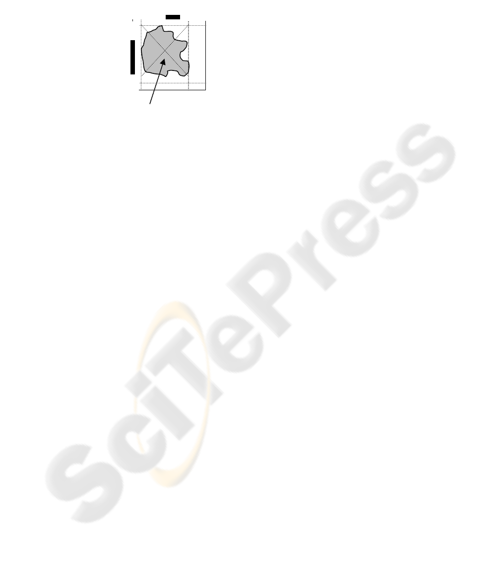
The last step consists in obtaining the trajectory of the objects by spatio-temporally
calculating the centroid (X
obj
, Y
obj
) of the maximally charged pixels of the moving
objects. Fig. 1 graphically shows the calculation of the centroid of an object.
Therefore the size is defined starting from the longitude of two right lines (or
cords) determined by four well-known pixels of the surface of the object [6]. The
pixels referenced this way are (x
1
, y
1
), (x
2
, y
2
), (x
3
, y
3
) and (x
4
, y
4
), such that:
yyyyxxxxtjiSyx >
<
>
<
∈∀
4321
,,,),,,(),( (5)
In other words, the four pixels are:
• (x
1
, y
1
) : pixel most at the left of the object in the image
• (x
2
, y
2
) : pixel most at the right of the object in the image
• (x
3
, y
3
) : upper most pixel of the object in the image
• (x
4
, y
4
) : lower most pixel of the object in the image
The two cords denominated maximum line segments of the object, won't unite the
214
pixels (x
1
, y
1
) and (x
2
, y
2
), (x
3
, y
3
) and (x
4
, y
4
) to each other, but rather their projec-
tions (X
1
, 0) and (X
2
, 0), (0 , Y
3
) and (0 , Y
4
), respectively, as you can appreciate in
Fig. 1.
X
2
X
1
Y
3
Y
4
(X
obj
, Y
obj
)
Fig. 1. Centroid of an object
Now, the object’s location will be determined by a unique characteristic pixel (X
obj
, Y
obj
), that is to say, the intersection of the two segments (X
1
, Y
3
)(X
2
, Y
4
) and (X
2
,
Y
3
)(X
1
, Y
4
). This centroid pixel will be denominated representative pixel of the object.
Once the maximum line segments and the representative pixel of an object have
been obtained in a sequence of images, it should be rather simple to detect a lot of
motion cases [7],[8]. Anyway, considering the following possibilities: no motion (N),
translation in X or Y-axis (T), dilation, or translation in Z-axis (D), and, rotation (R),
we may only obtain, by combining them, the following possibilities:
N no motion TDR translation + dilation + rotation
T pure translation D pure dilation
TD translation plus dilation DR dilation plus rotation
TR translation plus rotation R pure rotation
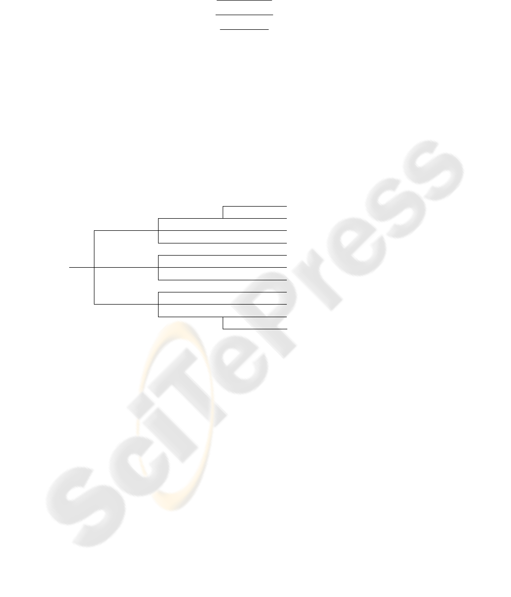
It is considered that the previous states appear in most cases (Fig. 2). Fig. 2 shows
the different possibilities when no change is detected in the representative pixels co-
ordinates enclosed in brackets. When there is a significant change in the co-ordinates
of the representative pixel, a T has been added enclosed in parenthesis. In this graph:
(1) Comparison between the horizontal maximum line segments of previous (k-1)
and current (k) image
(6)
⎪
⎩
⎪
⎨
⎧
<−−−
=−−−
>−−−
−
−
−
lXXXXifSmaller
lXXXXifEqual
lXXXXifLarger
kk
kk
kk
11212
11212
11212
)()(,
)()(,
)()(,
where l is the maximum permitted difference.
(2)
Comparison between the vertical maximum line segments of previous (k-1) and
current (k) image
(7)
⎪
⎩
⎪
⎨
⎧
<−−−
=−−−
>−−−
−
−
−
lYYYYifSmaller
lYYYYifEqual
lYYYYifLarger
kk
kk
kk
13434
13434
13434
)()(,
)()(,
)()(,
where l is the maximum permitted difference.
(3)
Similitude degree between the scale change of the maximum segments of im-
ages at k-1 and k
215
⎪
⎪
⎪
⎩
⎪
⎪
⎪
⎨
⎧
+≤
−
−
−
−
≤−
−
−
otherwiseDifferent
YY
YY
XX
XX
ifSimilar
k
k
k
k
,
1
)(
)(
)(
)(
1,
134
34
112
12
αα
(8)
where
α
is the permitted fluctuation in the similitude function.
(4)
Result state if the representative pixel of the object has not changed substan-
tially; a non substantial change is obtained by means of the following algorithm
)()(
11
dYYdXX
kobjkobjkobjkobj
≤
−
∩≤
−
−−
(9)
where d is the maximum permitted displacement.
(5)
Result state if the representative pixel of the object has changed substantially.
Of course, the possibility to offer some erroneous results with an unknown error
rate is assumed, especially in front of some rotation examples. Nevertheless, if the
number of images in a sequence is great enough, this error rate should be very little.
(1) (2) (3) (4) (5)
Similar [D] (TD)
Larger Different [DR] (TDR)
Larger Equal [R] (TR)
Smaller [R] (TR)
Larger [R] (TR)
Equal Equal [N] (T)
Smaller [R] (TR)
Larger [R] (TR)
Smaller Equal [R] (TR)
Smaller Similar [D] (TD)
Different [DR] (TDR)
Fig. 2. Motion states graph
2 Some Illustrative Examples
The algorithms exposed previously have been applied to multitude of synthetic se-
quences as shown in Fig. 3.
In example 1, a pure translation in one of the axis, in particular in the y-axis, is
shown. The algorithms work perfectly in this easy case (outputs is always D), even in
presence of the gleaned form of the treated object. Pure translations in the three axes
x, y , z have been all tested with this same and other synthetic objects. They have
offered the same good results in their behaviour. Evidently, it was expected that this
simple case had to work that well.
The second example is representative of more complex translation movements.
Here there are simultaneous translations in several axes. All possible translation com-
binations have been tested, obtaining for all the analysed objects an excellent behav-
iour of the algorithms. This concrete example offers the translation motion of an
216

irregular form in the three axes in a simultaneous way. That is the reason why the
correct result TD appears in all twenty steps of the approached synthetic sequence.
As it was easy to foresee, the problems would begin when incorporating rotational
movements. Example 3 is a sample of it. Indeed, we are in front of the case of a cube
approaching on z-axis and rotating simultaneously. Notice that the algorithm does not
throw the desired result DR, but a simple D, in the simulations. The explanation has
to be looked for in the shape of the object. Indeed, the algorithm works so much bet-
ter for the case of rotations the more irregular the shape of the analysed object’s mo-
tion is. Unfortunately, the horizontal and vertical segments always have the same
value for this figure.
Example 4 analyses a similar motion to the one of example 3. Here, nevertheless,
we are in front of an irregular shape. So it was waited to get a better behaviour of the
algorithms exposed in this work. And, indeed, good results are obtained from the
analysis of image 9 on of the sequence. The explanation of why the first images do
not throw the desired result is in the value chosen for the allowed fluctuation (
α
=0,2)
in the similitude function of the motion evaluation graph. A smaller value allows
improving the previous results.
(a) (b)
(c) (d)
Fig. 3. (a) Thumbtack sequence frames 1 and 20. (b) Irregular form sequence frames 1 and 20.
(c) Cube sequence frames 1 and 20. (d) Lamp sequence frames 1 and 20
4 Conclusions
In this paper, the LIAC model to spatio-temporally segment a moving object present
in a sequence of images has been introduced. In first place, this method takes advan-
tage of the inherent motion present in image sequences. This object segmentation
method may be compared to background subtraction or frame difference algorithms
in the way motion is detected. Then, a region growing technique is performed to
define the moving object. In contrast to similar approaches no complex image pre-
processing must be performed and no reference image must be offered to this model.
The method facilitates any higher-level operation by taking advantage of the common
charge value of parts of the moving object.
217

That is reason why it is so easy to introduce a simple but effective method for ob-
ject tracking. To some extent, the line of research on tracking using interframe match-
ing and affine transformations has been followed. Similarly to [9], the method de-
pends on the assumption that the image structure constrains sufficiently reliable mo-
tion estimation. Firstly, the detection of an important parameter of an object in move-
ment (its size) has been presented in this context. The algorithm is based on centroid
tracking [10]. Lastly, comparing the results obtained in the previous stage towards a
general graph for motion cases performs tracking. Compared to other approaches
based on geometric properties, the method proposed assumes that the images in the
sequences have a small transformation between them. Small changes over small re-
gions are also assumed. In this approach, the number of tracking features is kept to a
minimum. This permits to control one of the most important issues in visual systems:
time.
Acknowledgements
This work is supported in part by the Spanish CICYT TIN2004-07661-C02-02 grant.
References
1. D. Hogg, “Model-based vision: A program to see a walking person”, Image and Vision
Computing, vol. 1, no. 1, pp. 5-20, 1983.
2. J.L. Barron, D.J. Fleet, S.S. Beauchemin, “Performance of optical flow techniques”, Inter-
national Journal of Computer Vision, vol. 12, no. 1, pp. 43-77, 1994.
3. R. Jain, W.N. Martin, J.K. Aggarwal, “Segmentation through the detection of changes due
to motion”, Computer Graphics and Image Processing, 11, pp. 13-34, 1970.
4. M.A. Fernández, J. Mira, “Permanence memory: A system for real time motion analysis in
image sequences”, in IAPR Workshop on Machine Vision Applications, MVA’92, 1992,
pp. 249-252.
5. T.S. Huang, A.N. Netravali, “Motion and structure from feature correspondences: A re-
view”, Proceedings of the IEEE, 82, pp. 252-269, 1994.
6. R. Deriche, O.D. Faugeras, “Tracking line segments”, Image and Vision Computing, vol. 8,
no. 4, pp. 261-270, 1990.
7. A. Fernández-Caballero, Jose Mira, Ana E. Delgado, M.A. Fernández, “Lateral interaction
in accumulative computation: A model for motion detection”, Neurocomputing, 50C, 2003,
pp. 341-364.
8. A. Fernández-Caballero, J. Mira, M.A. Fernández, A.E. Delgado, “On motion detection
through a multi-layer neural network architecture”, Neural Networks, 16 (2), 2003, pp.
205-222.
9. M. Gelgon, P. Bouthemy, “A region-level motion-based graph representation and labeling
for tracking a spatial image partition,” Pattern Recognition, 33 (4), 2000, pp. 725-740.
10. G. Liu, R. M. Haralick, “Using centroid covariance in target recognition,” Proceedings
ICPR98, 1998, pp. 1343-1346.
218
