Petri-net modeling of production systems based on
production management data
Dejan Gradi
ˇ
sar and Ga
ˇ
sper Mu
ˇ
si
ˇ
c
1
Faculty of Electrical Engineering, University of Ljubljana, Tr
ˇ
za
ˇ
ska 25,
1000 Ljubljana, Slovenia
Abstract. Timed Petri nets can be used for the modeling and analysis of a wide
range of concurrent discrete-event systems, e.g. production systems. This pa-
per describes how to apply production management data and timed Petri nets
to the modeling of production systems. Information about the structure of a pro-
duction facility and about the products that can be produced is usually given in
production-data management systems. We describe a method for using these data
to algorithmically build a Petri-net model. The Petri-net model can be further
used to develop different analyses of the treated system.
1 Introduction
Any production management information system requires a detailed plan of production
operations. This can be achieved with a variety of software tools, which are capable of
(near optimal) scheduling the operations that are performed on different manufacturing
equipment, taking into account the finite number of available resources, precedence
constraints, etc.
In general, an adequate model of the production process is needed in order to de-
rive a feasible schedule that can be realized on the available manufacturing equipment.
Within the changing production environment the effectiveness of production modeling
is therefore a prerequisite for a successful scheduling system.
Petri nets (PN) represent a powerful graphical and mathematical modeling tool [9].
Many different extensions of classical PNs exist, and these are able to model a variety
of real systems. In particular, timed Petri nets can be used to model and analyze a wide
range of concurrent discrete-event systems [1], [4], [5], [14]. Several previous stud-
ies have addressed the timed Petri-net-based analysis of discrete-event systems. Lopez
[7], for example, deals with the simulation of the deterministic timed Petri net for both
timed places and timed transitions by using the firing-duration concept of time imple-
mentation. Petri nets can also be used in the design and operation of batch processes
[8]. Aalst [2] discusses the use of Petri nets in the context of workflow management.
There exists a lot of literature on the applicability of the PNs in the modelling, analysis,
synthesis and implementation of systems in the manufacturing applications domain. For
example, a comprehensive bibliography can be found in [15]. Authors in [10] show that
management strategies can be appropriately modeled by means of PNs. Strategies that
are considered in the article are push, pull and kanban strategy. Yu et al. [13] propose a
Gradišar D. and Muši
ˇ
c G. (2005).
Petri-net modeling of production systems based on production management data.
In Proceedings of the 3rd International Workshop on Modelling, Simulation, Verification and Validation of Enterprise Information Systems, pages 29-38
DOI: 10.5220/0002563900290038
Copyright
c
 SciTePress

new class of Petri nets, called Buffer nets, for modeling flexible manufacturing systems
(FMS). They present an approach that can build up a Petri net from a FMS specifica-
tion language. Tacconi [11] used the discrete-event matrix state equation together with
the Petri net state equation to obtain a complete dynamical description of a production
system.
A Petri-net model can be used to analyze a modeled system. Logical properties,
such as operability, the absence of deadlock, safety and hazards, etc. can be analyzed,
verified and validated. When time is integrated into PN models, quantitive performance
indices, such as cycle time, production rates and resource utilization, can be derived
and evaluated. With this analysis different possible task schedules can be evaluated.
The schedules obtained using PN theory are event-driven and deadlock free. Their other
feature is that the completition time or makespan criterion is the optimization objective.
The information about the structure of a production facility and about the products
that can be produced is usually given in the form of Manufacturing Resource Planning
(MRP II) which is a common way to express the production management systems.
With these systems an additional scheduling tool can be appended. In this configuration
the company can plan future activities while anticipating the market, but at the same
time being flexible enough to handle changes in the short term [3]. Czerwinski [6]
proposed a method for scheduling products with the bill of the material (BOM), using
an improved Lagrangian Relaxation technique. An approach presented by Yeh [12]
maintains production data by using a bill of manufacture (BOMfr), which integrates the
BOM and the routing data. Production data are then used to determine the production
jobs that need to be completed in order to meet demands.
Our work is based on using the data from production management systems where
the product structure is given in the form of the BOM and the process structure in the
form of routings. These two groups of data items, together with the work centers as
capacity units, form the basic elements of the manufacturing process. In this paper we
propose a method for using these data to automate the procedure of building up the
Petri-net model of a production system.
In the next section we describe timed Petri nets, where time is introduced by using
the holding-durations concept. Section 3 describes a method for modeling the basic
production activities with such a PN is described. In addition, the procedure for using
existing data from production-data management systems to build a model of an overall
production system is presented. Finally, the conclusions are presented in section 5.
2 Timed Petri nets
Petri nets are a graphical and mathematical modeling tool that is applicable to many
systems. Using Petri nets it is possible to study information-processing systems that are
characterized as being concurrent, asynchronous and parallel.
A Petri net is a bipartite directed graph with two types of nodes, called places and
transitions. Nodes are interconnected by directed arcs. State of the system is denoted by
distribution of tokens (called marking) over the places. A PN can be represented by the
multiple P N = (P, T, I, O, M
0
), where:
– P = (p
1
, p
2
, p
3
, ..., p
n
) is a finite set of places,
30

– T = (t
1
, t
2
, t
3
, ..., t
n
) is a finite set of transitions,
– I : (P × T ) → N is the input arc function. If k input arcs connect p
j
to t
i
, then
I(p
j
, t
i
) = k.
– O : (P × T ) → N is the output arc function. If k output arcs connect t
i
to p
j
, then
O(p
j
, t
i
) = k.
– M
0
: P → N is the initial marking.
A transition t
j
is enabled by a given marking if, and only if, M (p
j
) > I(p
j
, t
i
) for
all p
j
∈ P . An enabled transition can fire, and as a result remove tokens from input
places and create tokens in output places. If the transition t
j
fires, then the new marking
is given by M
′
(p
j
) = M (p
j
) + O(p
j
, t
i
) − I(p
j
, t
i
).
An important concept in PNs is that of conflict. Conflict occurs between transitions
that are enabled by the same marking, where the firing of one transition disables the
other transition. Also, concurrency (parallel activities) can easily be expressed in terms
of a PN. A situation where conflict and concurrency are mixed is called a confusion.
The concept of time is not explicitly given in the original definition of Petri nets.
However, for the performance evaluation and scheduling problems of dynamic sys-
tems it is necessary to introduce time delays. As described in [4], there are three basic
ways of representing time in Petri nets: firing durations, holding durations and enabling
durations. The names given to Petri nets augmented with time vary greatly from one
researcher to another. Time delays can be assigned to places or transitions. Given that
a transition represents an event, it is natural that time delays should be associated with
transitions. Holding durations work by classifying tokens into two types, available and
unavailable. Available tokens can be used to enable a transition, whereas unavailable
tokens cannot. To each transition a time duration is assigned, and when firing occurs,
the action of removing and creating tokens happens instantaneously. However, the cre-
ated tokens are not available to enable new transitions until they have been in their
output place for the time specified by the transition that created them. This principle is
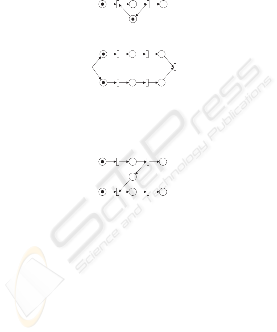
graphically represented in Figure 1.
t =2
p
t =2
p
t =2
p
0t <
2t0 <£
t2 £
Fig.1. Timed Petri net with holding durations
By using holding durations the formal representation of the timed Petri net is ex-
tended with the information of time, represented by the multiple P N = (P, T, I, O, M
0
,
T imestamp, T ime
t), where:
– P, T, I, O, M
0
are the same as above,
– T imestamp : P → 2
R
+
0
. To each place p
i
∈ P a set of non-negative real numbers
is associated, representing timestamps of tokens residing in the place.
– T ime
t : T → R
+
0
is the function that assigns to each transition t
i
∈ T a time
delay.
31

To each transition fixed time delay is associated as described with T ime t function.
The state of a timed Petri net is given by the distribution of tokens over the places and
the corresponding timestamps of the tokens. To each token a non-negative real number
(timestamp) is associated, which defines for how many time units the token remains
unavailable. Available token has a timestamp with value 0. In any time interval, the
marking is defined with M = M
a
+ M
u
, such that M
a
is made of available and M
u
of unavailable tokens. A transition t
j
is enabled by a given marking if, and only if
M
a
(p
j
) > I(p
j
, t
i
) for all p
j
∈ P . The firing of transitions is considered instantaneous.
The model remains at a given model time as long as there are enabled transitions. A new
marking is determined and the timestamps of tokens remain unchanged, while newly
produced tokens receive the timestamps as prescribed with transitions that produced
them. When no more transitions are enabled at the current time, the time is incremented
as defined with the time increment. The values of timestamps are decremented for that
value until enabling condition is satisfied again.
3 The modeling of production activities
In this section the modeling of production activities using timed Petri nets is presented.
Many classes of PN can be used to describe production process like state machines,
marked graphs, assembly Petri nets, etc., which can be used to describe production
processes [15]. Aalst, in his work [4], provides a method for mapping scheduling prob-
lems onto timed Petri nets, where the standard Petri-net theory can be used. To support
the modeling of scheduling problems, he proposed a method to map tasks, resources
and constraints onto a timed Petri net. In this paper a different representation of time in
Petri nets is used.
Here we present the method of describing the production system activities with
timed Petri nets using the holding-duration representation of time. The places repre-
sent resources and jobs/operations, and the transitions represent decisions or rules for
resources assignment/release and starting jobs.
As it can be seen from Figure 1 operation can be described with one place and two
transitions. The transition t determines the processing time of an operation. During that
time the created token is unavailable in place p.
An operation possibly needs resources, usually with a limited capacity, to be exe-
cuted; this is illustrated in Figure 2. The token in place p
R1
gives information about
the availability of the resource. When the resource begins with the execution the un-
available token appears in place p
1op
. After the time defined by transition t
1in
the token
becomes available and the resource becomes free to operate on the next job. For this
reason zero time needs to be assigned to transition t
1out
. To be able to define the time
for the next operation place p
1
is added. There are common situations where more oper-
ations use the same resource, e.g. an AGV, mixing reactor. In that case the place noting
the resource is connected to all those operations. Similarly, there are situations where a
particular operation can be done on two different resources. This is represented as two
coupled operations, between places p
0
and p
1
.
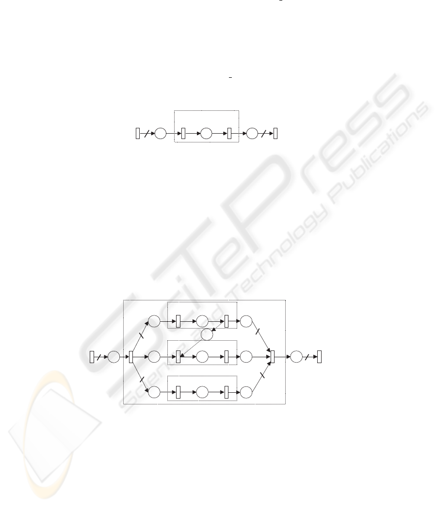
When parallel activities need to be described the Petri-net structure presented in
Figure 3 is used. Transitions t
11in
and t
12in
define the duration of each operation.
32

p
0
t=2
1in
p
1op
p
1
p
R1
t
1out
Fig.2. Operation that uses a resource with finite capacity
p
01
p
02
t
11in
t
12in
p
11op
p
11
p
12
t
11out
t
12out
p
12op
t
1
t
0
Fig.3. Two parallel operations
Precedence constraints are modeled by adding an extra place. Figure 4 shows the
situation where the task presented with p
1op
precedes the task presented with place
p
2op
.
p
01
p
02
t=2
1in
t=3
2in
p
1op
p
1
p
2
p
pr1
t
1out
t
2out
p
2op
Fig.4. Precedence constraint
In Petri-net modeling, the place nodes can be used to represent the status of a re-
source (e.g., its availability), the stage of a process plant operation (e.g., undergoing)
and a condition (e.g., its satisfaction). The presence of a token in a place indicates if
a resource is available, a process plant operation is undergoing, or a condition is true
(e.g., material is available). Transition nodes are used to model events, e.g., the starting
and ending of an operation.
4 Modeling using the data from production management systems
In a production management system, e.g. MRP II, the product structure is given in the
form of the BOM and the process structure in the form of routings. These two groups
of data items together with the work centers as capacity units, form the basic elements
of the manufacturing process. These data can be effectively used to build up a model of
the production system with Petri nets. Here we provide a method for recognizing basic
33

production elements from the management system’s database and using them to build
up a Petri-net model of this production system.
The BOM is a listing or description of the raw materials and items that make up
a (semi)product, along with the required quantity of each. It can be represented as
BOM = (R, E, q, pre), where:
– R is a root item,
– E are sub-items,
– q are quantities of required items,
– pre is precedence constraints matrix. pre(i, j) = 1 indicates that i-th item precedes
j-th item.
If any of the sub-items E is composed of any other sub-items, the same definition
is used to describe its dependencies. Listings of all the items which appear in a product
define the BOM structure of a product.
I
J
K L
3 1 2
M
J
L
2
1
a) b)
Fig.5. BOM structure of product I (a) and its component M (b)
In Figure 5a there is an example of a BOM describing the production of product I.
It is composed of three components, i.e. 3 items of J, one K item and two items of L.
From the graph it is clear that item J has to be completed before the production of item
K can begin – see dotted line. The BOM of product I would be represented as:
BOM = (R, E, q, pre), where
R =

I

, E =

J K L

, q =

3 1 2

and pre =


0 1 0
0 0 0
0 0 0


.
Each of sub-items (in our case J, K or L) can be composed of sub-items from a
lower level. In this case this sub-item represent a root item in the next BOM, defining
from which sub-items is consisted from.
Each item from BOM is represented with a Petri-net structure P N
Ei
. This structure
is represented graphically in Figure 6. Item I is represented with the nodes t
Iin
, p
Iop
and
t
Iout
. To be able to prescribe how many of each item is required the transition t
Rin
and
the place p
Rin
are added in front, and p
Rout
and t
Rout
are added behind this structure.
The weight of the arcs that connect t
Rin
and p
Rin
and p
Rout
and t
Rout
determine the
quantity q of the required items. In this way an item is represented with a timed PN
defined as:
34

P N
E
i
= (P, T, I, O, M
0
, T imestamp, T ime
t), where
P = {p
R
in
, p
I
op
, p
R
out
}, T = {t
R
in
, t
I
in
, t
I
out
, t
R
out
}, I =


0 1 0 0
0 0 1 0
0 0 0 q


,
O =


q 0 0 0
0 1 0 0
0 0 1 0


,
M
0
(p
i
) = 0, T imestamp(p
i
) = ∅, ∀p
i
∈ P ,
and T ime
t(t
i
) = 0, ∀t
i
∈ T .
ItemI
p
Rin
t
Iin
p
Iop
p
Rout
t
Iout
t
Rin
q
t
Rout
q
Fig.6. PN structure representing one item in the BOM
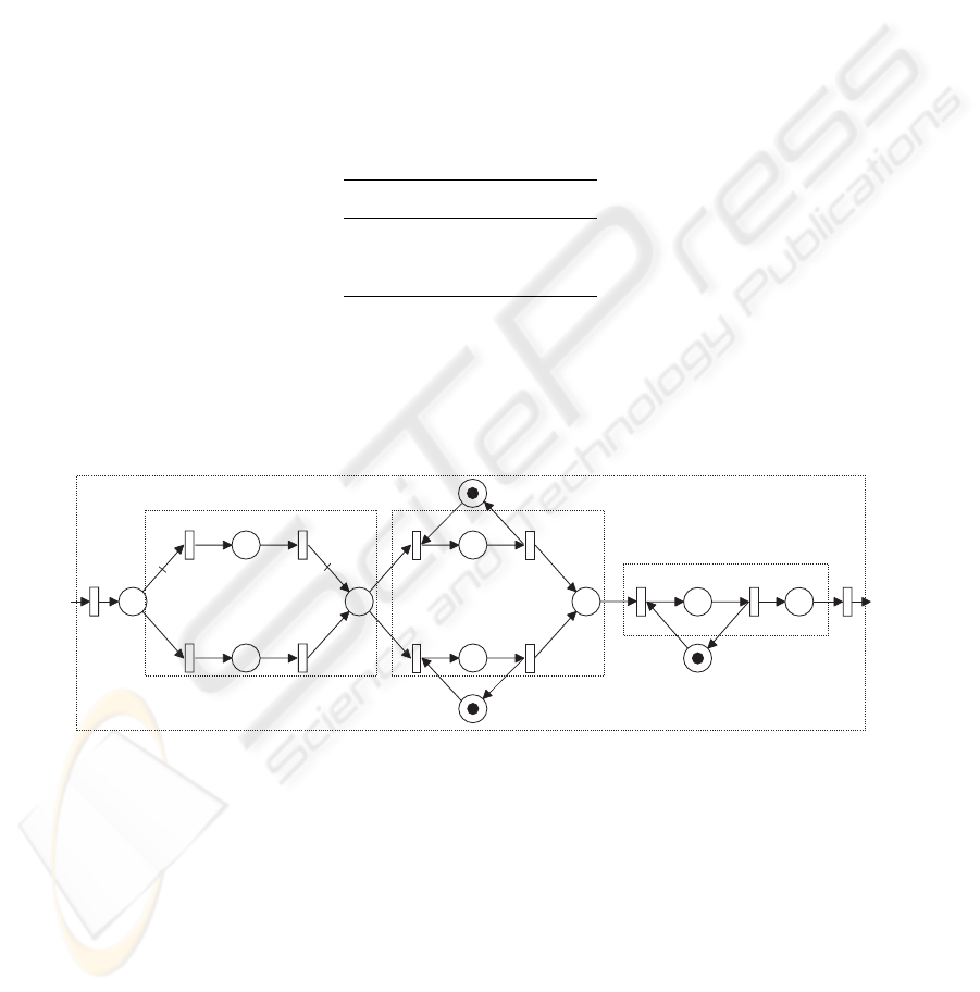
The construction of the overall Petri net is an iterative procedure that starts with
the root of the BOM and continues until all the items have been considered. If the item
requires any more sub-assemblies (i.e. items from a lower level) the item is substituted
with lower-level items. If there are more than one sub-items, they are given as parallel
activities. In Figure 7 the P N
Ei
structure of the previous example is given, where item
I is composed of three sub-items: J, K and L. When one item had to be produced before
another, the precedence constraints had to be introduced. In our case item J had to be
finished before the production of item K could begin.
t
Jin
p
Jop
t
Kin
t
Lin
p
Kop
p
Lop
p
t
Rin
p
Rin
t
Iin
p
IinJ
p
IinK
p
IinL
p
IoutJ
p
IoutL
p
IoutK
t
Iout
t
Rout
Rout
q
q
2
3
p
Pr
ItemJ
ItemL
ItemK
ItemI
2
3
t
Jout
t
Kout
t
Lout
Fig.7. Example of PN structure defined from the BOM
For each item that can appear in the production process the routing shows the se-
quence of production operations and associated work centers. The processing times are
associated with each of the operations.
Each operation that appears in the routing represent basic production activity. Their
Petri-net representations are placed in the model. Some of their representations are de-
35

scribed in previous section. The time durations of the operations are assigned to the
transitions depicted as t
in
. All the placed operations are connected as prescribed by the
required technological sequence.
The required resources are assigned to the operations. Each resource that exists in
the facility is represented by a place. If there are more operations that need the same
resource, they are all connected to the place representing that resource. The capacity of
a resource is demonstrated by the number of tokens in it.
A routing for item K is presented in Table 1. Three operations are needed to produce
this item; the third takes 12 seconds, using the resource R3 and the second operation
can be done on two different resources, but the first operation is defined with a product
M. The structure of this semi-product is defined with a BOM described in Figure 5b.
Table 1. Routing of item K
Operations Duration Resources
Op10 – M
Op20 10s (9s) R1 (R2)
Op30 12s R3
The PN structure in Figure 8 is achieved if the sequence of operations described
with a previous routing is modeled.
p
K10
t
t
p
K1Lop
p
K1Nop
t
t
p
K1
p
K3op
t 12= t
p
K3
P
R1
Op10-ItemM
Op30
t
Kin
t
Kout
ItemK
K1Lin
K1Nin
K1Lout
K1Nout
K3in K3out
P
R3
t =10
t
p
K21op
p
K22op
t =9
t
p
K2
P
R2
Op20
K21in
K22in
K21out
K22out
2
2
Fig.8. Routing of item K modeled with timed Petri net
In this a way the routings are submodels that are inserted into the main model de-
fined with the BOM. However, these sub-items can also be described with a BOM as it
can be seen from the example in the case of first operation - Op10. The construction of
the overall Petri-net model can be achieved by combining all of the intermediate steps.
Products to be produced and required quantities of finished products are determined
by a work order (WO). A Petri-net model is build for each product as defined with BOM
36

and routing data. At the end the Petri-net model should be verified and simplified, if pos-
sible. The modeling procedure can be summarized in the following algorithm:
Algorithm 1
[R, q] = readWO()
For i = 1 to length(R)
PN = placePN(R(i), [], q(i), [])
PN = routing(PN, R(i))
end
First, data about the WO are read. The products which are needed to be produced
are given in vector R and in vector q the quantities of the desired products are passed.
For each product first the Petri-net structure P N
Ei
(see Figure 6) is determined and
placed on the model. The weight q is assigned to the corresponding arcs. The step when
the routing() is called is described in more detail with algorithm 2:
Algorithm 2
function routing(PN, R)
[E, q, pre] = readBOM(R)
datRoute = readRouting(R)
for i = 1 to length(datRoute.Op)
if datRoute.Resources ==BOM
PN1 = placePN(R, E, q, pre)
for j = 1 to length(E)
routing(PN, E(j))
PN = insertPN(PN, PN1)
end
else
PN = construct
PN(PN, datRoute)
end
end
First, the routing and the BOM data are read from the database. For each operation
that compose the routing, algorithm checks if it is made up of sub-item(s). If this is the
case, function placePN() is used to determine the PN structure of a given BOM, see
Figure 7. For each of those sub-items the routing data need to be implemented. With
function insertPN() the resulted subnet is inserted in the main PN. If the operation repre-
sents the production operation function constructPN() is called. With it basic elements
(Figures 2– 4) are recognized and placed in the model. All the data about resources
and time durations are acquired from the routing table. A prototype of the described
algorithm has been implemented in Matlab.
37

5 Conclusion
Production management data and timed Petri nets with the holding-duration principle
were used to model production activities. In production management systems the prod-
uct structure is usually given in the form of the BOM and the process structure in the
form of routings. These two groups of data items, together with the work centers as
capacity units, form the basic elements of the manufacturing process. A procedure for
using existing data from production management systems to build the Petri-net model
was developed.
The proposed method is an effective way to get an adequate model of the production
process, which can be used to develop different analyses of the treated system, e.g.
schedules. The intention of the future work is to make some additional tests of the
provided method on the real manufacturing environment.
References
1. van der Aalst, W.M.P.: Petri net based scheduling. Computing Science Report, 23 (1995)
2. van der Aalst, W.M.P.: The Application of Petri nets to Workflow Management. Journal of
Circuits Systems and Computers, 8(1), (1998) 21–66.
3. Berning, G., Brandenburg, M., G
¨
ursoy, K., Kussi, J.S., Mehta, V., T
¨
olle, F.: Integrating col-
laborative planning and supply chain optimization for the chemical process industry (I) -
methodology. Computers and Chemical Engineering, 28, (2003) 913–927.
4. Bowden, F. D. J.: A brief survey and synthesis of the roles of time in Petri nets. Mathematical
& Computer Modelling, 31, (2000) 55–68.
5. Freedman, P.: Time, Petri nets, and robotics. IEEE Transactions on Robotics and Automation,
7(4), (1991) 417–433.
6. Czerwinksi, C. S., Luh, P. B.: Scheduling products with Bills of materials using an improved
lagrangian relaxation technique. IEEE Tr. on robotics and automation, 10(2), (94) 99–111.
7. L
´
opez-Mellado, E.: Analysis of discrete event systems by simulation of timed Petri net mod-
els. Mathematics and Computers in Simulation, 61, (2002) 53–59.
8. Gu, T., Bahri. P. A.: A survey of Petri net applications in batch processes. Computers in
Industry, 47, (2002) 99–111.
9. Murata, T.: Properties, analysis and applications. Proc. of the IEEE, 77(4), (1989) 541–580.
10. Recalde, L., Silva, M., Ezpeleta, J., Teruel, E., Petri Nets and Manufacturing Systems: An
Examples-Driven Tour. In: Lectures on Concurrency and Petri Nets, Vol. 3098. Springer-
Verlag (2004), 742-788.
11. Tacconi, D. A.: A New Matrix Model for Discrete Event Systems: Application to Simulation.
Control Systems Magazine, IEEE, 17, (1997) 62–71.
12. Yeh, C.H.: Schedule based production. International Journal of Production Economics, 51,
(1997) 235–242.
13. Yu, H., Reyes, A., Cang, S., Lloyd, S.: Combined Petri net modelling and AI based heuristic
hybrid search for flexible manufacturing systems-part 1. Petri net modelling and heuristic
search. Computers & Industrial Engineering, 44, (2003) 527–543.
14. Zuberek, W. M., Kubiak, W.: Timed Petri Nets in Modeling and Analysis of simple Schedules
for Manufacturing Cells. Comp. and Mathematics with Applications, 37, (1999) 191–206.
15. Zhou, M. C., Venkatesh, K., Modelling, Simulation, and Control of Flexible Manufacturing
Systems: A Petri Net Approach (World Scientific) (1999)
38