
A New RBF Classifier for Buried Tag Recognition
Larbi Beheim, Adel Zitouni and Fabien Belloir
CReSTIC
(Centre de Recherche en Sciences et Technologies de l’Information et la Communication)
University of Reims Champagne-Ardenne
Campus du Moulin de la Housse, B.P. 1039,
51687 Reims Cedex 2, France
Abstract. This article presents noticeable performances improvement of an
RBF neural classifier. Based on the Mahalanobis distance, this new classifier
increases relatively the recognition rate while decreasing remarkably the num-
ber of hidden layer neurons. We obtain thus a new very general RBF classifier,
very simple, not requiring any adjustment parameter, and presenting an excel-
lent ratio performances/neurons number. A comparative study of its perform-
ances is presented and illustrated by examples on real databases. We present
also the recognition improvements obtained by applying this new classifier on
buried tag.
1 Introduction
The radial basic functions neural net (RBF) has become, for these last years, a serious
alternative to the traditional Multi-Layer Perceptron network (MLP) in the multidi-
mensional approximation problems. RBF Network was employed since the Seventies
under the name of potential functions and it is only later than [1] and [2] rediscovered
this particular structure in the neuronal form. Since, this type of network profited
from many theoretical studies such as [3], [4] and [5]. In pattern recognition, RBF
network is very attractive because its locality property allows discriminating complex
classes such as nonconvex ones.
We consider in this article the Gaussian RBF classifier of which each m output s
j
is
evaluated according to the following formula:
()()
1
11
1
() () exp
2
hh
NN
T
jljllj ll
ll
sX w X w XC X C
ϕ
−
==
l
⎧
⎫
==−−Σ−
⎨
⎬
⎩⎭
∑∑
(1)
Where X=[x
1
… x
n
]
T
∈
R
N
is a prototype to be classified, Nh represents the total num-
ber of hidden neurons. Each one of these nonlinear neurons is characterized by a
center C
l
∈R
N
and a covariance matrix
Σ
l
.
From a training set S
train
={X
p
,
ω
p
}, p=1…N made up of prototypes couples X
p
and
its membership class
ω
p
∈
{1…,m}, the supervised training problem of RBF classifier
amounts determining his structure, i.e. the number of hidden neurons Nh and the
Beheim L., Zitouni A. and Belloir F. (2005).
A New RBF Classifier for Buried Tag Recognition.
In Proceedings of the 5th International Workshop on Pattern Recognition in Information Systems, pages 22-32
DOI: 10.5220/0002562800220032
Copyright
c
SciTePress

different parameters intervening in the equation of outputs (1). Whereas these pa-
rameters can be calculated by different heuristics, the estimate of Nh is often delicate.
For that, many methods were developed among which we can quote [6], [7] and [8].
These methods generally require a very significant load of calculation without how-
ever guaranteeing significant performances. Moreover, they often require a certain
number of parameters that must be fixed a priori and optimized for a particular prob-
lem. So these methods cannot be applied systematically and without particular pre-
cautions to any type of classification problem. The article [9] proposed a very simple
algorithm, which generates automatically a powerful RBF network without any opti-
mization nor introduction of parameters fixed a priori. Indeed, the algorithm auto-
matically selects the number of the hidden layer neurons. Although this network is
characterized by its great simplicity, it presents a major limitation however owing to
the fact that it requires a rather significant number of neurons in the hidden layer.
This limitation makes it very heavy and requiring very significant training times for
the very large databases.
In this article we propose a solution to this problem by introducing the Mahalano-
bis distance. We thus obtain a new very general, very simple RBF network and pre-
senting an excellent performances/neurons number ratio. We present also the recogni-
tion improvements obtained by applying this new classifier on buried tag coding
system.
The organization of the article is as follows: In section 2, we describe the new RBF
network and we present the associated algorithm. Its operation is illustrated for an
example on an artificial database. In section 3, we study its properties and in section 4
its performances on real problems. Finally, we present results obtained by application
of this classifier on buried tag coding system.
2 Algorithm
In this section, we describe the principle of construction proposed as well as the algo-
rithm allowing its implementation. We illustrate then his operation in a problem of
classification including two classes of which one is not convex.
2.1 Principle
The principle of the algorithm rests on [9]. According to the exponential nature of the
functions
ϕ
l
(.) of each hidden neuron, the activation state of each one of them de-
crease quickly when the vector of entry X moves away from the neuron center. So
only an area of the entry space centered in C
l
will provide a significantly non-null
activation state. Contrary to [9], our algorithm regards this area as a hyperellipsoide
centered in C
l
. Indeed, the use of the Mahalanobis distance makes it possible to take
into account the statistical distribution of the prototypes around the centers C
l
and
thus a better representation of classes shape. Our algorithm proposes to divide a non-
23

convex class into a set of hyperellipsoides called clusters. Each cluster corresponds to
a hidden neuron and it is characterized thus by a center placing it in the entry space, a
matrix of covariance indicating the privileged directions and a width calculating the
extension of the hyperellipsoide. In the continuation, we will not make any more the
distinction between a neuron and a cluster.
2.2 Description
Before describing the construction algorithm of the RBF classifier, we will introduce
some notations used thereafter. At the k
th
iteration, we define C
(k)
ij
like the i
th
center
(i=1… m
(k)
j
) characterizing the class
Ω
j
. With each center a covariance matrix is asso-
ciated
Σ
(k)
ij
and a width L
(k)
ij
. We note H
(k)
ij
the hyperellipsoide of center C
(k)
ij
such as:
(
)
(
)
{
}
() ()1
,
T
kk
ij p j p ij ij p ij ij
H X XC XC L
−
=∈Ω − Σ −<
(2)
Each class is characterized by the area R
(k)
j
defined as the union of all the hyperel-
lipsoides H
(k)
ij
(i=1… m
(k)
j
).
We will also use the distance d(R
(k)
j
,X) between a point X
∈Ω
j
and its associated
area R
(k)
j
. This one is defined as the Mahalanobis distance between X and the nearest
center C
(k)
ij
of R
(k)
j
:
()
(
)
(
)
)()(
min,
1
)(
1
)(
)(
k
ij
k
ij
XRd
CXCX
k
ij
T
mi
k
j
k
j
−
∑
−
−
=
=
K
(3)
Step 0 (initialization): For k=0, we define m clusters whose centers correspond to
the gravity centers of different classes
Ω
j
(N
j
is the element number of
Ω
j
) :
m
(0)
j
=1 and
∑
Ω∈
==
jpX
p
j
j
mjX
N
C K1,
1
)0(
1
()()
mjCXCX
N
jpX
T
j
p
j
p
j
j
K1,
1
1
)0(
1
)0(
1
)0(
1
=−−
−
=∑
∑
Ω∈
(4)
(5)
Step 1 (adjustment of the widths): The width L
(k)
ij
relating to the center C
(k)
ij
is de-
fined like the half of Mahalanobis distance between this center and the nearest center
of another class :
()()
()
()
() () () ( 1)1 () ()
,1
1,1
1
min
2
k
t
k
j
T
kkkk
ij ij st ij ij st
tjs m
imjm
LCCC
−−
≠=
==
=−Σ
K
KK
kk
C−
(6)
Step 2 (search for an orphan point): We seek a point X
i
∈
S
train
not belonging to its
associated area R
(k)
ω
i
and most distant from this one:
24

(
)
s
k
SX
i XRdX
s
trains
,max arg
)(
ω
∈
=
(7)
If such a point does not exist, go to the step 5.
Step 3 (creation of a new center): Point X
i
found at step 2 becomes a new center
composing the class
Ω
ω
i
:
1
)()(
+=
k
j
k
j
mm
i
k
jm
XC
k
j
=
)(
,
)(
(8)
Step 4 (Reorganization of the centers): The K-means clustering algorithm is ap-
plied to the points of S
train
pertaining to the class
Ω
ω
i
in order to distribute as well as
possible the m
(k)
j
centers. Calculate the new covariance matrices:
()()
()
() () ()
()
1
()1
k
pij
T
kk
ij p ij p ij
k
XH
ij
XC XC
Card H
∈
Σ= − −
−
∑
k
T
(9)
Do k=k+1 and go to the step 1.
Step 5 (determination of the weights): The weights matrix W
*
which minimizes an
error function, here selected as the sum square errors of classification, and is given
by:
1
* TT
WHHH
−
=
⎡⎤
⎣⎦
(10)
where H and T are the matrices respectively gathering the activation function stats
and the target outputs. These last are fixed at 1 when they correspond to the class of
the point and 0 elsewhere.
2.3 Discussion
The initialization of the algorithm (step 0) could have proceeded by the random
placement of a number of given centers. This technique is very current in the defini-
tion of an RBF network. The fact of choosing the initial centers as gravity centers of
the points X
p
makes it possible to avoid this unforeseeable character and provides
moreover the number of these centers. Thus, the result of the algorithm depends only
on the composition of the training data. In certain cases where the classes are non
convex, it may be that the gravity center of a class is inside another class. This situa-
tion is not prejudicial for the algorithm since this center will be moved during follow-
ing iterations.
The covariance matrix corresponding to each center is obtained from
the associated training data. We will further see that other definitions of this matrix
can give different results. In step 1, L
(k)
ij
is defined relatively to the minimal distance
between the center C
(k)
ij
and centers of another class. This means that a partial cover-
ing between the clusters of the same class is authorized. From a practical point of
view, that makes it possible to optimize the space occupation of the attributes by the
various zones of
receptivity and thus to reduce the number of clusters necessary to
compose each class. The elliptic volume covered by each cluster is maximal without
25
encroaching on neighboring classes. In step 2, the fact of choosing the furthest point
from the region R
(k)
j
makes it possible to improve the effectiveness of the algorithm of
K-means clustering used at step 4. It should be noted that this one relates only to the
centers constituting the same class since the other centers did not change a position. It
guarantees moreover a fast development of this area. In the network training (step 5),
the target outputs are fixed arbitrarily at 1 when they correspond to the class of the
point and 0 elsewhere. The motivation of this practice is artificially to create a brutal
fall of the membership degree at the geometrical border of the class.
After k iterations, all the points of Strain belong to a cluster, the algorithm gener-
ated m+k clusters defining as many subclasses. The RBF network thus built com-
prises then Nh=m+k hidden neurons. We can note that the algorithm converges nec-
essarily. Indeed, in the "worst case" where none the classes is separable, there will be
creation of a cluster for each point of Strain.
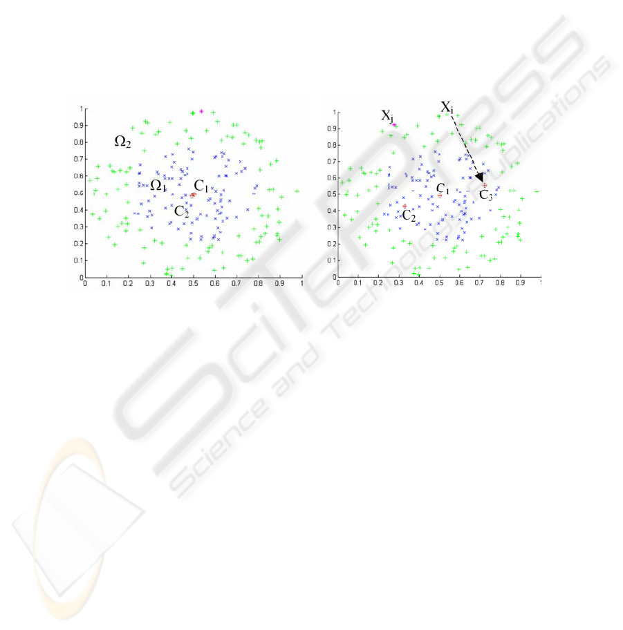
Fig. 1. Algorithm initialization.
Fig. 2. 1st iteration of the algorithm.
2.4 Illustration of operation
We will illustrate the significant phases of the algorithm on a classification problem
of two concentric classes from the databases of "ELENA" project [10] [11]. This base
makes it possible to determine the capacity of a classifier to separate two classes not
overlapping but of which one is included in the second.
The RBF network comprises 2 inputs and 2 outputs. The figure 1a shows the 2
initial centers {C
1
,C
2
} obtained following step 0. We can see that the two centers are
almost confused. Each cluster induced is delimited by an ellipse of the width
calculated at step 1. Obviously, the cluster of center C
2
is not sufficient to entirely
represent the class
Ω
2
. This one thus will be subdivided in several subclasses. With
the first iteration of the algorithm, the point noted X
i
on the figure 2 is the furthest
from the center C
2
and is out of the corresponding cluster. The addition of a new
center compared to this point led, after application of the K-means, to the new distri-
26
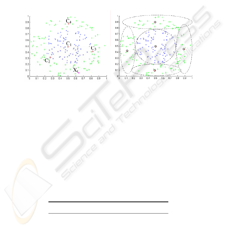
bution {C
1
,C
2
,C
3
} illustrated by the figure 2. The point X
j
is now the furthest from the
center C
3
on this figure. After application of the K-means on this new configuration
one leads to the figure 3. After 4 iterations, the 2 classes are discriminated perfectly
and the neuronal classifier comprises a total of 5 neurons (see figure 4). After having
determined the number of centers necessary and their positions, the weights of the
network are calculated according to equation of step 5. The algorithm thus manages
to separate the two classes with only 5 neurons against 108 neurons for the old algo-
rithm using the Euclidean distance and with a slightly higher rate of recognition: 98%
against 97.7% for the old RBF.
C
1
C
2
C
3
C
4
C
5
C
1
C
2
C
3
C
4
C
5
Fig. 3. 2nd iteration of the algorithm.
Fig. 4. Result of classification of the algo-
rithm.
2.5 The choice of the covariance matrix
One of the limits of this classifier is the estimate of the covariance matrix. The larger
the size of the clusters is and the better is the estimate of this matrix. So the calcula-
tion of this matrix can sometimes reduce the rates of recognition. To cure this prob-
lem, other calculations of this matrix can be proposed to take into account more pro-
totypes during the estimate of this matrix.
Table 1 gives examples of calculation, errors and the corresponding number of neu-
rons. One can see on this table that a different choice of the covariance matrix that
proposed in section 2 can increase or decrease the rate error but the number of hidden
neurons can only increase. But this number remains always largely lower than the
number of neurons proposed by the old RBF.
Table 1. Error rate of the base Textures according to the choice of the matrix of covariance
Covariance Matrix
a
Error(%) Nh
Σ=cov(C) (a) 2,90 24
Σ=cov(Ji) (b) 1,94 3
27
Σ=cov(JCi) (c) 1,73 858
Σ=cov(J) (d) 0,41 22
a
(a) covariance of the centers, (b) covariance of the data of each class (c) covariance of the data
of each center (d) covariance of the total database.
3 Benchmarks
The object of this section is to evaluate the performances of the RBF classifier built
by the algorithm presented in section 2. For that, we applied the classifier to various
problems of classification comprising a variable number of attributes and classes and
bearing from the real world situations.
3.1 Pima Indians Diabetes Database
This database is from the Machine Learning database repository at the University of
California, Irvine [12]. In this problem there are two classes representing results of a
diabetes test given to Pima Indians. There are 8 attributes, and 768 examples, ran-
domly partitioned into two disjoint subsets of equal size for training and testing. Ta-
ble 2 presents comparative results of different classifiers (backpropagtion networks,
decision trees or support vector machines [13],…). For more details on methods of
this table see [14].
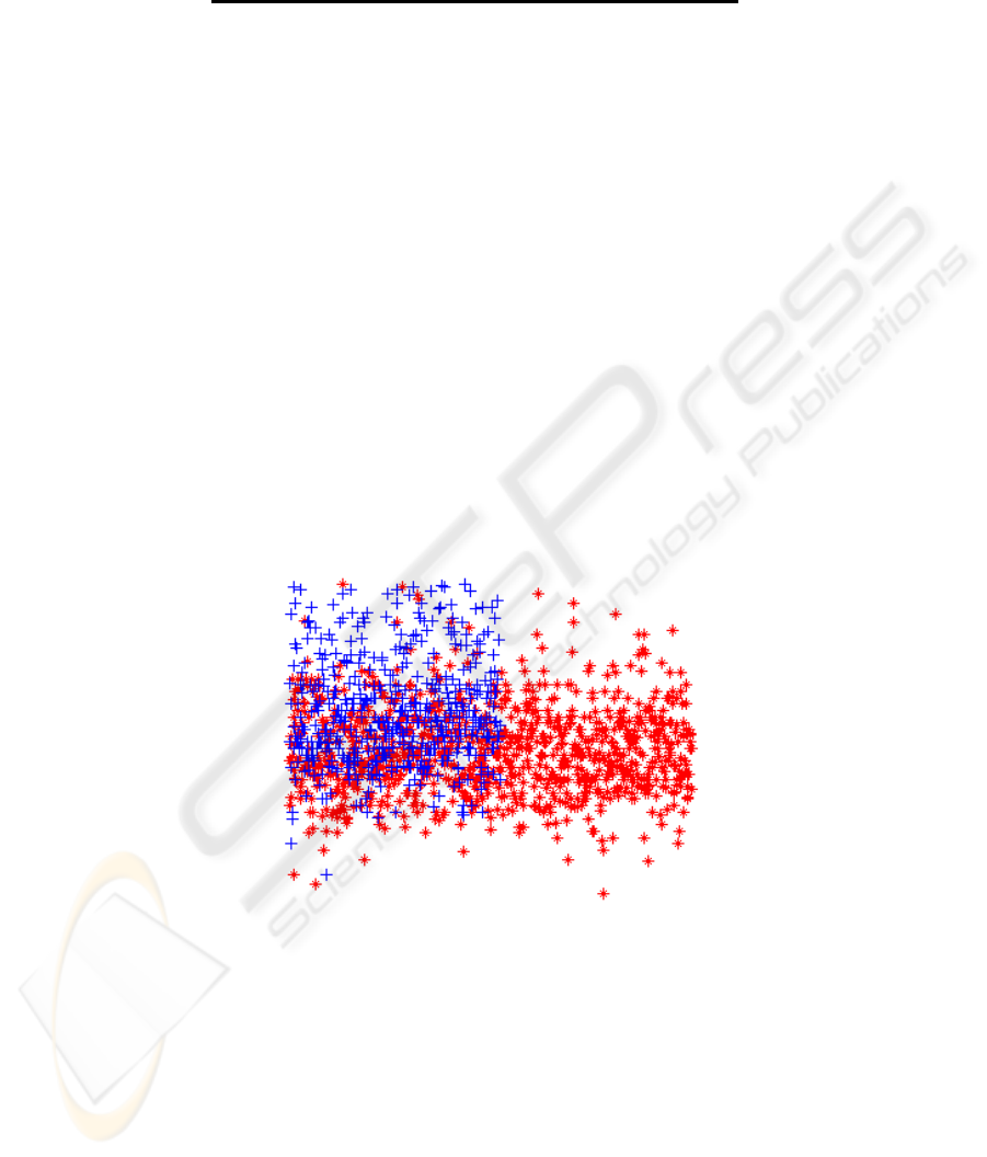
Fig. 5.
Pima Indians database (2 first attributes)
We can see on this example, the RBF classifier gives the weakest error rate (with
the Linear MSE classifier). The relatively high error rate (23%) and the number of
hidden neurons (76 units) is due to the fact that this database comprises partially
superimposed classes (see Figure 5).
28

Table 2. Pima Indians Database Results
Method Error rate (%)
Linear MSE (pseudoinverse) 23
Oblique Decision Tree 8 decision nodes 24
1-1 Nearest Neighbor 30
2-3 Nearest Neighbor 25
Full covariance gaussian mixture, 1 component/class 26
Full covariance gaussian mixture, 2 component/class 29
Full covariance gaussian mixture, 3 component/class 30
Full covariance gaussian mixture, 4 component/class 31
Backprop Multilayer Perceptron 2 hidden units 25
Backprop Multilayer Perceptron 4 hidden units 24
Backprop Multilayer Perceptron 8 hidden units 29
Support Vector Machine, RBF kernel, width 1 (297 s.v.) 30
Support Vector Machine, RBF kernel, width 3 (176 s.v.) 35
Support Vector Machine, polynomial kernel, order 4 (138 s.v.) 36
Support Vector Machine, polynomial kernel, order 5 (131 s.v.) 34
MFGN 4 components 35
MFGN 6 components 32
MFGN 8 components 35
Our RBF classifier (76 hidden units) 23
3.2 ELENA Databases
The benchmarks carried out here are studied in detail in ELENA project [10]. The
three databases result from real problems. The "Phoneme" problem relates to the
speech recognition. The principal difficulty of this problem is great dissymmetry in
the number of authorities of each classes. The "Iris" data is very known in the pattern
recognition. To finish, the data of the "Texture" file relates to the recognition of 11
natural micro-textures such as grass, sand, paper or certain textiles. For each problem
of classification, we have the results concerning the RBFM classifier generated by the
algorithm proposed, the RBFE is the classical RBF classifier based on Euclidian
distance and other classifiers studied in [11]. The table 3 presents results on these
various problems. The performances of the RBF classifier are slightly lower than the
other classifiers for the first problem. This is explained by the significant interlacing
of the two classes. The algorithm generates a neuron number close to the point’s
number of training data and the capacities of generalization on the test set are thus
very bad.
Table 3. Error rate (%) and hidden neuron number (Nh) on four different databases
Method Phoneme Iris Texture
KNN 12.90 3.50 2.20
MLP 16.10 4.10 2.10
LVQ 17.10 6.10 3.40
RBFE (Euclidian)
10.90
Nh=227
2.90
Nh=24
1.80
Nh=858
29

RBFM (Mahalanobis)
10.43
Nh=59
1.94
Nh=3
0.41
Nh=22
The error rate of our classifier RBFM is generally the weakest for each of the last
three problems. This is checked whatever the number of classes to be distinguished
and the quantity of available data for the training.
We can see on this table the "compact" quality of our classifier who gives compa-
rable error rates or even lower while minimizing the hidden neurons number Nh. So,
training times are much less significant. For the "Textures" database for example, the
error rate is divided by 4, while the number of hidden neurons is divided by 39. It was
necessary less than two minutes to training our classifier and more than one hour for a
classical RBFE classifier.
4 Application in buried tag identification
The goal of our application is to detect and identify reliably different buried metallic
codes with a smart eddy current sensor. Based on the principle of the induction bal-
ance, our detector measures the magnetic fields modifications emitted by a coil.
These modifications are due to the presence of the metal codes buried on the top of
the drains. A code is built from a succession of different metal pieces separated by
empty spaces. Thus the identification of the codes allows the identification and the
localization of the pipes (like water, gas,…) [15].
Several material improvements were carried out on our detector [16], but the iden-
tification of the codes always poses problems because of the similarity between the
codes, the non-linearity of the answer according to the depth and the choice of a suit-
able coding of the signals [17]. To solve these problems, various methods of classifi-
cations were proposed. These methods are based on neural networks. Among all
developed methods it is the classifier RBFE (Euclidean RBF) who gives the best
results. But, these results remain insufficient for the great depths. It is for that we
developed this new classifier to try to decrease rate errors and neurons number for a
future integration of the classifier on programmable microchips. A comparison is
made between these different methods and the new RBF classifier. For a burying
depth up to 80 cm, we obtain the results given in the table 4. We can notice that the
result of the new RBF classifier is better than the others, and always with less number
of hidden neurons.
Table 4. Results of code misclassification for the 5 pattern recognition methods implemented
Classifier
a
RBFM RBFE SOM
Error (%) 5.0 6.2 11.3
Nh 68 135 80
a
RBFM=RBF based on Mahalanobis distance, RBFE= RBF based on Euclidian distance, SOM=Self Or-
ganization Map.
30

5 Conclusion
We proposed a noticeable performances improvement of a neural classifier based an
RBF network. The new classifier is very general and simple. It generates automati-
cally a powerful RBF network without any introduction of parameters fixed a priori.
The number of hidden neurons is very optimized what will allow its use for the very
large databases. Indeed, the new classifier obtains excellent recognition results for a
variety of different databases and particularly the buried tag recognition. On this
application we can also note a reduction in the error rate (relatively weak) but espe-
cially a very clear reduction in the number of hidden neurons (division by 2). This
allows a notable saving of the training times necessary to the development of the
system.
References
1. D.S. Broomhead and D. Lowe, Multivariable functional interpolation and adaptive net-
works, Complex Systems, Vol.2, 1988, pp. 321-355.
2. J. Moody and C.J. Darken, Fast Learning in Networks of Locally-Tuned Processing Units.
Neural Computation, Vol.1, 1988, pp. 281-294.
3. F. Girosi and T. Poggio, Networks and The Best Approximation Property, Technical Re-
port C.B.I.P. No. 45, Artificial Intelligence Laboratory, Massachusetts Institute of Tech-
nology, 1989.
4. Park J. and Sandberg I.W., Universal Approximation Using Radial-Basis-Function Net-
works, Neural Computation, Vol.3, 1991, pp. 246-257.
5. M. Bianchini, P. frasconi and M. Gori, Learning without Local Minima in Radial Basis
Function Networks, IEEE Transactions on Neural Networks, Vol.6:3, 1995, pp. 749-756.
6. B. Fritzke, Supervised Learning with Growing Cell Structures, In Advances in Neural
Processing Systems 6, J.C. Cowan, Tesauro G. and Alspector J. (eds.), Morgan Kaufmann,
San Mateo, CA., 1994.
7. B. Fritzke, Transforming Hard Problems into Linearly Separable one with Incremental
Radial Basis Function Networks, In M.J. Vand Der Heyden, J. Mrsic-Flögel and K. Weigel
(eds.), HELNET International Workshop on Neural Networks, Proceedings Volume I/II
1994/1995, VU University Press, 1996
8. C.G. Looney, Pattern Recognition Using Neural Network - Theory and Algorithms for
Engineers and Scientits, Oxford University Press, Oxford - New York, 1997.
9. F. Belloir, A. Fache and A. Billat, A General Approach to Construct RBF Net-Based Clas-
sifier, Proc. of the European Symposium on Artificial Neural Networks (ESANN’99),
April 21-23, Bruges Belgium, 1999, pp. 399-404.
10. C. Aviles-Cruz, A. Guerin-Dugué, J.L. Voz and D. Van Cappel, Deliverable R3-B1-P Task
B1: Databases, Technical Report ELENA ESPRIT Basic Research Project Number 6891,
June 1995.
11. F. Blayo, Y. Cheneval, A. Guerin-Dugué, R. Chentouf, C.Aviles-Cruz, J. Madrenas,
M. Moreno and J.L. Voz, Deliverable R3-B4-P Task B4: Benchmarks, Technical Report
ELENA ESPRIT Basic Research Project Number 6891, June 1995.
12. Merz, C.J. and Murphy, P.M. (1996). UCI Repository of machine learning databases.
[http://www.ics.uci.edu/~mlearn/MLRepository.html]. Irvine, CA: University of Califor-
31

nia,
Department of Information and Computer Science.
13. F. Friedrichs, C. Igel, Evolutionary Tuning of Multiple SVM Parameters, Proceedings of
the 12th European Symposium on Artificial Neural Networks (ESANN 2004), Evere, Bel-
gium, 2004.
14. A. Ruiz, P. E. López-de-Teruel, M. C. Garrido, Probabilistic Inference from Arbitrary
Uncertainty using Mixtures of Factorized Generalized Gaussians, Journal of Artificial In-
telligence Research 9, pp. 167-217, 1998.
15. F. Belloir, F. Klein and A. Billat, Pattern Recognition Methods for Identification of Metal-
lic Codes Detected by Eddy Current Sensor, Signal and Image Processing (SIP'97), Pro-
ceedings of the IASTED International Conference, 1997, pp. 293-297.
16. L. Beheim, A. Zitouni, F. Belloir, Problem of Optimal Pertinent Parameter Selection in
Buried Conductive Tag Recognition, Proceedings of WISP’2003, IEEE International Sym-
posium on Intelligent Signal Processing, Budapest (Hungary), 4-6 September 2003, pp. 87-
91.
17. F. Belloir, L. Beheim, A. Zitouni, N. Liebaux, D. Placko, Modélisation et Optimisation
d'un Capteur à Courants de Foucault pour l'Identification d'Ouvrages Enfouis, 3e Colloque
Interdisciplinaire en Instrumentation (C2I’2004), Cachan (France), 29-30 janvier 2004.
32
