
VISUAL SVM
François Poulet
ESIEA – Pôle ECD, 38, rue des Docteurs Calmette et Guérin, 53000 Laval, France
Keywords: Visual Data Mining, Support Vector Machine, High Dimensional Datasets, Cooperative Approach
Abstract: We present a cooperative approach using bo
th Support Vector Machine (SVM) algorithms and visualization
methods. SVM are widely used today and often give high quality results, but they are used as "black-box",
(it is very difficult to explain the obtained results) and cannot treat easily very large datasets. We have
developed graphical methods to help the user to evaluate and explain the SVM results. The first method is a
graphical representation of the separating frontier quality (it is presented for the SVM case, but can be used
for any other boundary like decision tree cuts, regression lines, etc). Then it is linked with other graphical
methods to help the user explaining SVM results. The information provided by these graphical methods can
also be used in the SVM parameter tuning stage. These graphical methods are then used together with
automatic algorithms to deal with very large datasets on standard personal computers. We present an
evaluation of our approach with the UCI and the Kent Ridge Bio-medical data sets.
1 INTRODUCTION
The size of data stored in the world is constantly
increasing but data do not become useful until some
of the information they carry is extracted.
Furthermore, a page of information is easy to
explore, but when the information reaches the size of
a book, or library, or even larger, it may be difficult
to find known items or to get an overview.
Knowledge Discovery in Databases (KDD) can be
defined as the non-trivial process of identifying
valid, novel, potentially useful, and ultimately
understandable patterns in data (Fayyad et al., 1996).
In this process, data mining can be defined as the
p
articular pattern recognition task. It uses different
algorithms for classification, regression, clustering
or association. In usual KDD approaches,
visualization tools are only used in two particular
steps: in one of the first steps to visualize the data or
data distribution, in one of the last steps to visualize
the results of the data mining algorithm, between
these two steps, automatic data mining algorithms
are carried out.
Some new methods have recently appeared
(W
ong, 1999), trying to involve more significantly
the user in the data mining process and using more
intensively the visualization (Shneiderman, 2002),
this new kind of approach is called visual data
mining. We present some graphical methods we
have developed to increase the visualization part in
the data mining process and more precisely in
supervised classification tasks.
The first method is used to evaluate the quality
an
d interpret or explain the results of Support Vector
Machine (SVM) algorithms used in supervised
classification. Very few papers have addressed this
topic (Caragea et al, 2003), (Poulet, 2002). In
supervised classification SVM algorithms have
shown to be very efficient but they are used as "a
black box". We have an accurate model of the data,
but no explanation about this model and most of the
time this is what the end-user is waiting for. The
SVM is able to classify a new data point in class +/-
1, but we do not know why.
A first graphical method is used to give the user
an
evaluation of the quality of the obtained
separating surface. This first graphical method is
then linked with another one to try to explain what
are the attributes having an important part in the
classification.
Then we show how we can also use the
i
nformation given by this kind of visualization
method to help the user in tuning the SVM algorithm
parameters. Parameter tuning is a very important
part of the data mining task (with SVM algorithms
and with many other ones), but here again the
process is nearly never described. Our approach
doesn't solve the whole problem but only avoid
parsing all the possibilities and when we are dealing
with very large datasets (one million data points or
more) this can be really time saving.
309
Poulet F. (2005).
VISUAL SVM.
In Proceedings of the Seventh International Conference on Enterprise Information Systems, pages 309-314
DOI: 10.5220/0002521003090314
Copyright
c
SciTePress
One restriction of the data visualization methods
is well known: they usually cannot treat very large
data sets. At last, we present a cooperative approach
using both the previous graphical method and
automatic algorithms to efficiently deal with very
large datasets.
2 SVM ALGORITHMS
SVM algorithms (Vapnik, 1995) are kernel-based
methods used for supervised classification,
regression or novelty detection and have been
successfully applied to a large number of
applications. Let us consider a linear binary
classification task, with m data points in the n-
dimensional input space R
n
, denoted by the x
i
(i=1,…, m), having corresponding to labels y
i
= ±1.
For this problem, the SVM try to find the best
separating plane, i.e. furthest from both class +1 and
class -1. It can simply maximize the distance or
margin between the support planes for each class
(x.w – b = +1 for class +1, x.w – b = -1 for class -1).
The margin between these supporting planes is
2/||w||. Any point falling on the wrong side of its
supporting plane is considered to be an error.
Therefore, the SVM has to simultaneously maximize
the margin and minimize the error. The standard
SVM formulation with linear kernel is given by the
following quadratic program (1) where slack
variables z
i
≥ 0 and constant C > 0 is used to tune
errors and margin size.
Min f (w, b, z) = (1/2) ||w||
2
+ C Σ z
i
s.t. y
i
(w.x
i
– b) + z
i
≥ 1 (1)
z
i
≥ 0 (i=1, …, n)
The plane (w,b) is obtained by the solution of the
quadratic program (1). And then, the classification
function of a new data point x based on the plane is:
f(x) = sign (w.x – b).
SVM can use some other classification
functions, for example a polynomial function of
degree d, a RBF (Radial Basis Function) or a
sigmoid function. To change from a linear to non-
linear classifier, one must only substitute a kernel
evaluation in (1) instead of the original dot product.
More details about SVM and others kernel-based
learning methods can be found in (Cristianini, 2000).
Recent developments for massive linear SVM
algorithms (Fung and Mangasarian, 2001)
reformulate the classification as an unconstraint
optimization and these algorithms require thus only
solution of linear equations of (w,b) instead of
quadratic programming. If the dimensional input
space is small enough (less than 10
4
), even if there
are millions of data points, the new SVM algorithms
are able to classify them in minutes on a PC (Poulet
and Do, 2003). The algorithms can deal with non-
linear classification tasks however the m
2
kernel
matrix size requires very large memory size and
execution time. Reduced support vector machine
(RSVM) (Lee and Mangasarian, 2000) creates a
rectangular kernel matrix of size mxs (s << m) by
using a small random data points S being a
representative sample of the entire dataset and
reduces the size problem. The authors have proposed
some possible ways to choose S from the entire
dataset. However, most of existing SVM algorithms
have two disadvantages: they are used as "black-
box", it may be difficult to explain the results
obtained and they need a important parameter tuning
stage before to give the expected accuracy.
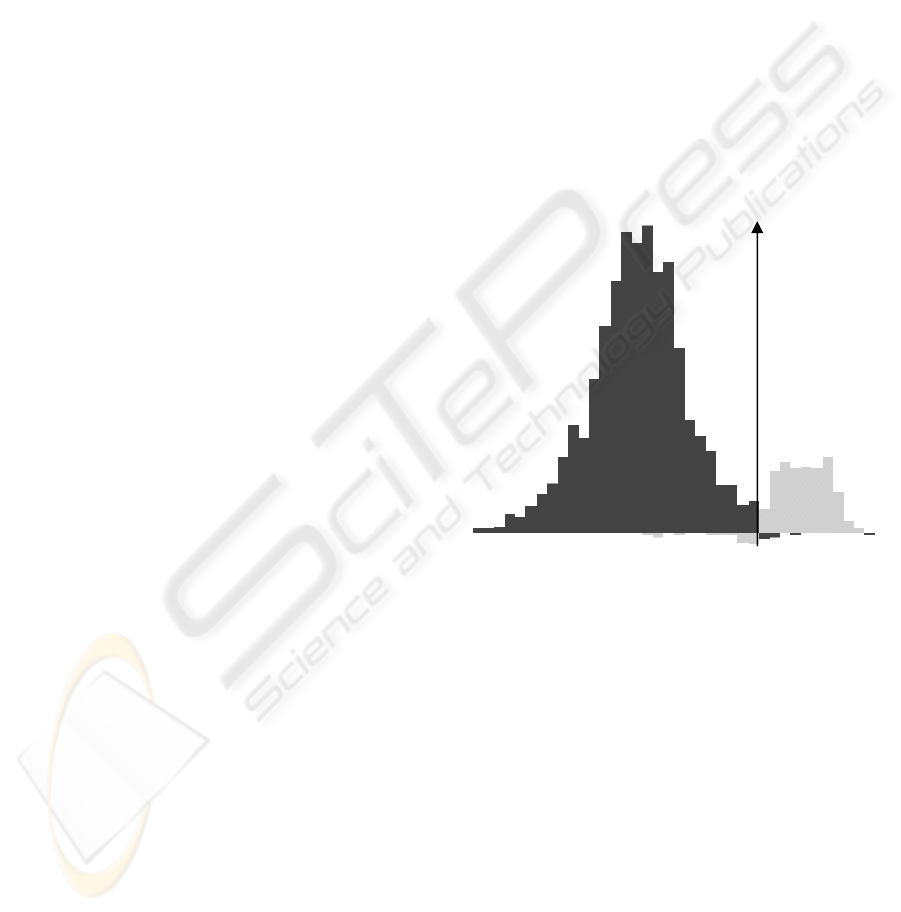
Figure 1: Distribution of the segment data points, class
5 against all.
3 GRAPHICAL INTERPRETATION
OF SVM RESULTS
We have developed a graphical method in order to
try to explain the SVM results and evaluate their
quality. The first step of our algorithm is to compute
the data distribution according to the distance to the
separating surface. While the classification task is
performed we also compute this distance for every
data point.
ICEIS 2005 - ARTIFICIAL INTELLIGENCE AND DECISION SUPPORT SYSTEMS
310
For each class, the positive distribution is the set
of correctly classified data points, and the negative
distribution is the set of misclassified data points.
Then we display this distribution by the way of a
simple histogram. We can use this single tool to
evaluate the quality of the separating frontier. It can
be used for SVM separating boundary or any other
separating feature (like a cut in a decision tree
algorithm or a regression line). Figure 1 shows an
example of such a distribution with the class 5 of the
Segment data from the UCI Machine Learning
Repository (Blake and Merz, 1998).
We can see the separating frontier (here a plane
because we used a linear kernel) is a good one: there
are only some misclassified data points (negative
distribution) near the separating frontier (the vertical
axis). Another possibility is to use this tool linked
with other data representations, for example a set of
two-dimensional scatter plot matrices (Becker et al,
1987) or parallel coordinates (Inselberg and Avidan,
1999). Figure 2 shows an example of a set of scatter-
plot matrices. They are the 2-dimensional
projections of the data according to all possible pairs
of attributes. One of the two-dimensional matrices is
selected and displayed in a larger size in the bottom
right part of the visualization.
When the user selects a bar in the graphical
distribution, the corresponding data points are
selected in the other graphical tools too. For example
if we select the bars nearest from the separating
plane, the corresponding points are selected in the
scatter plot matrices too. This allow the user to have
some interesting information about the boundary
between the two classes: what are the important
attributes for the classification, is it a straight
frontier or is it a complex one, etc.
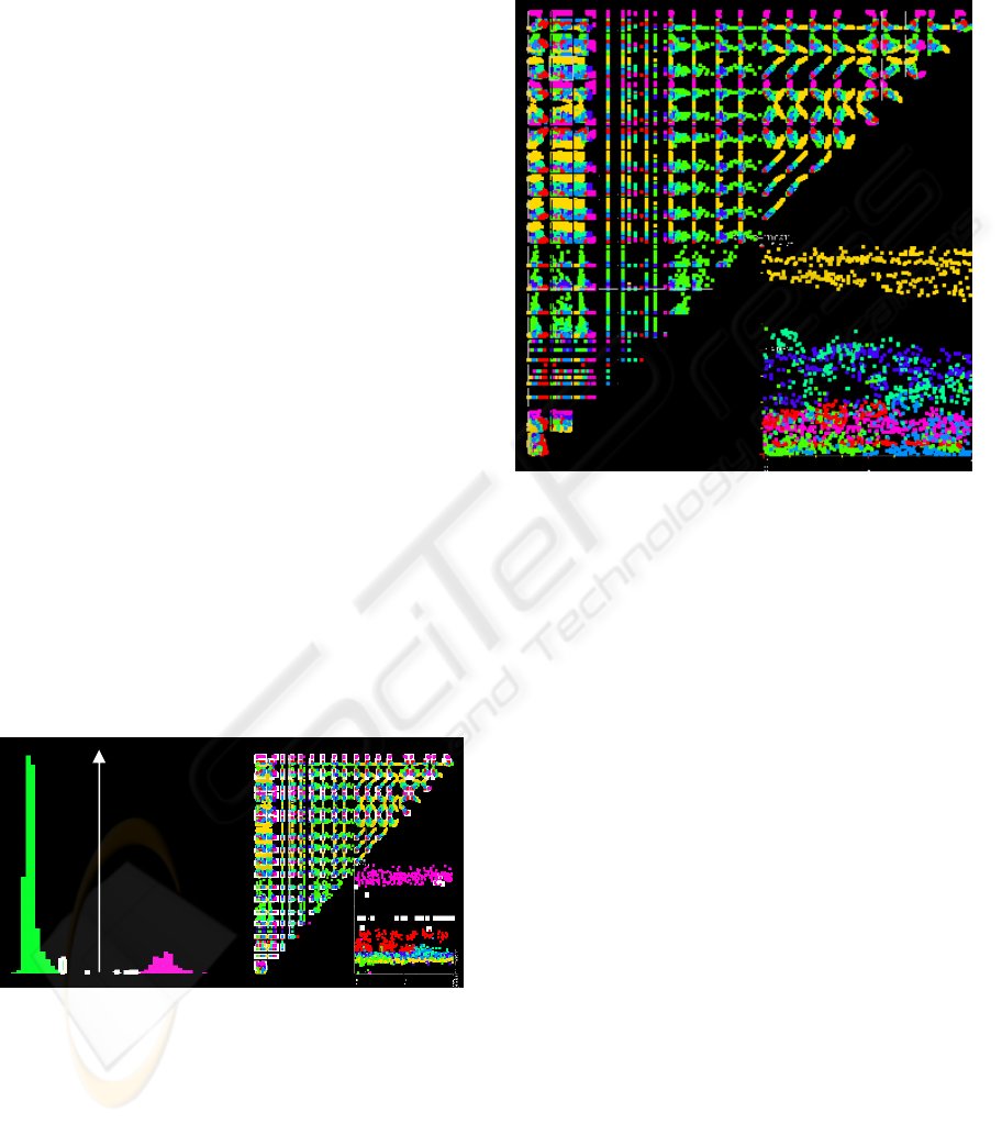
Figure 2: Scatter-plot matrices display of the Segment
dataset.
Figure 3 shows an example of a straight frontier
between the class 7 and the other ones (always in the
Segment dataset). We can see on the distribution of
the data according to their distance to the separating
hyper-plane, there is no data point near the
boundary. We select the nearest from the boundary,
and these points are automatically selected in the set
of scatter plot matrices in the right of Figure 3 (the
selected elements are in bold white). We find again
the same information as in the distribution display:
there is no point near the boundary (there is a wide
empty space between the class 7 and the other ones).
Figure 3: Visualization of the separating hyper-plane
between class 7 and the other ones in the Segment dataset.
But we have more information than the quality
of the boundary, we have also information about its
shape and about the attributes important for the
current class. Figure 3 shows the boundary between
the class 7 and the other ones is a straight line. And
we can also infer from the visualization that the two
attributes corresponding to the x and y axes in the
bottom right part of the visualization are the ones
deciding the membership of class 7. In this particular
case it is even simpler, the boundary is a horizontal
line: only the attribute corresponding to the y-axis
(hue-mean) is important for the class 7 (in a decision
tree, we would have a node like: (if (hue-mean < x)
then class=7).
It is possible to link the graphical distribution
with any other graphical representation.
This simple graphical tool allows us to explain
the results obtained by a SVM algorithm. The
graphical representation of the data distribution
according to their distance to the separating frontier
gives a good idea of its quality. It is true for a SVM
separating hyper-plane and for any other frontier
(like a cut in a decision tree or a regression line,
etc.).
Furthermore, when linked with another graphical
data representation (for example the scatter-plot
matrices or the parallel coordinates), the distribution
can help the user in interpreting the frontier: he is
able to explain what is the attribute(s) that make(s) a
VISUAL SVM
311

point belonging to a given class. One must not forget
nearly all SVM algorithms only give the accuracy
and the support vectors (n-dimensional vectors for a
n-dimensional dataset). With this kind of results it is
impossible to explain anything in the obtained
classification (even if it gives a high quality
accuracy). The comprehensibility and confidence in
the result are never used in algorithm evaluation but
an end user will not use a model if he has not a
minimum comprehension and confidence in it.
The scatter-plot matrices and parallel-
coordinates are only useful if the number of
dimensions (database columns) and the number of
items (database rows) are limited to some dozens of
dimensions and some thousands of items. We will
address this point in section 5.
4 GRAPHICAL SVM PARAMETER
TUNING
Parameter tuning is a very important part of the
SVM algorithms even if very few papers explain
how to perform this task. We call parameter either
the tuning of the algorithm input parameter, either
the choice of the kernel function.
One paper (Fung et al, 2002) explains how to
perform this task. This is an exact citation from this
paper:
"Following the methodology used in prior work,
we tested our algorithm on this dataset together with
the knowledge sets, using a "leave-one-out" cross-
validation methodology in which the entire training
set of 106 elements is repeatedly divided into a
training set of size 105 and a test set of size one. The
values of
ν
and
µ
associated with both KSVM and
SVM1 were obtained by a tuning procedure which
consisted of varying them on a square grid: {2
-6
, 2
-
5
,…, 2
6
}x{2
-6
, 2
-5
,…, 2
6
}."
For someone who is not a SVM expert (and even
sometimes for the experts), the only way to get high
quality results is to perform several classification
tasks with parameters varying in the good range
values.
We can use the information obtained by the
visualization tools described in the previous section
to help the user.
A first possibility is to use the results of the data
distribution according to their distance to the
separating frontier. In the example shown in Figure
3 (left part), we can see there is no data point near
the frontier. This gives the user the following
information: at least one parameter has not to be
tuned finely. This simple information can really
reduce the time needed for the classification task.
This will not change the classification accuracy,
only the time needed to perform it.
Another possibility is to use the data
visualization to help the user choosing the kernel
function. In the examples shown in figure 2 and
figure 3, we can see a linear boundary between the
elements of the class 2 and class 7. So a linear kernel
function will be sufficient to get good results.
Conversely we cannot conclude anything if we
cannot see a linear boundary: if the frontier between
two classes is an n-dimensional hyper-plane, any
projection on two attributes will not show this
frontier. But the visualization of the data distribution
according to their distance to the separating hyper-
plane can give us this kind of information: if for
example, there are several misclassified data points
near the boundary, another kernel function may be
more suitable.
Another interesting feature is to use these tools
for the multi-class case. SVM algorithms are only
able to deal with two classes. When the dataset has
more than two classes the most used approaches are
the one-against-all and the one-against-one. A set of
classifiers is built and then the classification of a
new item is performed with a vote mechanism. The
same kernel function and the same parameters
tuning are used for the whole treatment. Here, we
can use the visualization methods to help the user to
tune parameters and to choose a kernel function for
each class and so use sophisticated (with often high
computational cost) kernel function only when
needed. The visualization is used to guide the user in
his choices and reduce the number of classification
algorithms to run.
We have seen how simple visualization methods
can help the user to evaluate the quality of the result
obtained by an automatic SVM algorithm and
interpret or understand this result on one hand, and
to help him to choose the parameters or kernel
functions to use to get great results without having to
execute several times the classification algorithm on
the other hand.
5 COOPERATIVE METHODS
As mentioned in section 3, the scatter-plot matrices
and parallel-coordinates are only useful if the
number of dimensions (database columns) and the
number of items (database rows) are limited to some
dozens of dimensions and some thousands of items.
In order to be able to deal with larger datasets, we
combine automatic algorithms and visualization
algorithms to get a cooperative method able to deal
with large datasets.
ICEIS 2005 - ARTIFICIAL INTELLIGENCE AND DECISION SUPPORT SYSTEMS
312
5.1 Dimensionality reduction
Some applications have to deal with datasets having
very large number of dimensions (for example in
text-mining or bioinformatic). Most existing
classification algorithms cannot deal with such
datasets and use a pre-processing step to reduce the
dataset dimensionality.
To deal with these datasets, we use a feature
selection method with the 1-norm linear SVM
proposed by (Fung and Mangasarian, 2004) as data
preprocessing. The 1-norm linear SVM algorithm
maximizes the margin by minimizing 1-norm
(instead of 2-norm with standard SVM) of plane
coefficients (w). This algorithm provides results
having many null coefficients. The corresponding
dimensions are removed, this can efficiently select
few dimensions corresponding to non-null
coefficients without losing too much information.
We have evaluated the performances of the
algorithm on the bio-medical datasets from the Kent
Ridge Bio-medical Data Set Repository (Jinyan and
Huiqing, 2002).
After a feature selection task with the 1-norm
linear SVM, we have used the LibSVM to classify
these datasets. The results concerning the accuracy
are shown in table 1: the accuracy is equal or
increased for four datasets and reduced in only one
case. So may be, we can talk about dimensionality
selection (like for the nested cavities described in
(Inselberg and Avidan, 1999)) instead of
dimensionality reduction. And then, visualization
tools are able to work on these datasets.
This cooperative approach allows the user to
interpret the results of SVM algorithms dealing with
datasets having a very large number of attributes.
5.2 Data reduction
In order to deal with datasets having large number of
items (rows of the database) we use the same kind of
approach as the RSVM algorithm.
First, we use a k-means algorithm to create
clusters and then we sample data points from the
clusters. The resulting small dataset is then
displayed with scatter-plot matrices and the user
interactively selects the subset S of points (used as
support vectors in input of the RSVM algorithm).
These points are the points closest to the separating
boundary between the two classes.
We illustrate our approach with the UCI Forest
cover type dataset (581,012 data points, 54
dimensions and 7 classes). This dataset is known as
a difficult classification problem for SVM
algorithms. (Collobert et al, 2002) trained the
models with SVMTorch and a RBF kernel using
100,000 training data points and 50,000 testing data
points. The learning task needed more than 2 days
and 5 hours with an accuracy being 83.24 %. We
have also classified the class 2 against all, we have
used 500,000 data points for training and the rest to
test. LibSVM was not able to finish the learning task
after several days. To use our cooperative approach
with this dataset, about 1 hour was needed to create
200 clusters (100 for each class) and sampling 5,000
data points (25 points/cluster). Then, we have
interactively selected support vectors from the
reduced dataset in a set of scatter-plot matrices as
shown in figure 4. A rectangular RBF kernel was
created in input of RSVM. The learning task needed
about 8 hours for constructing the model with an
accuracy equal to 83.77%. This is a first promising
result of our tool on large datasets.
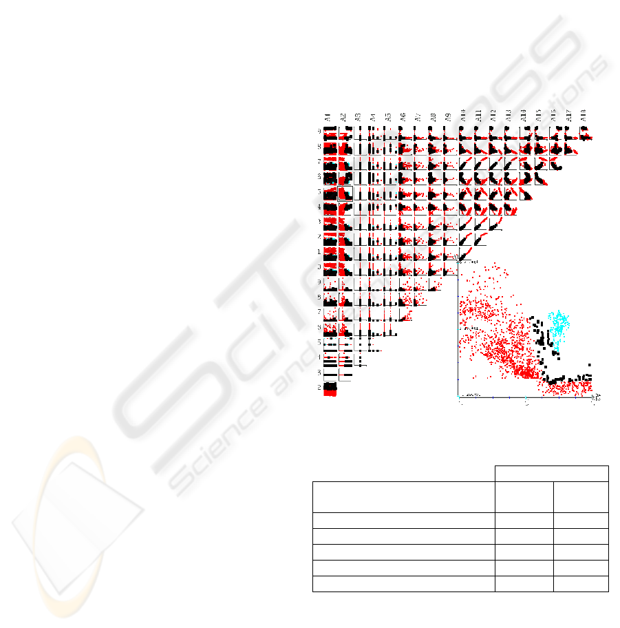
Figure 4: Interactive support vector selection for the
Segment class 6
Table 1: Accuracy with and without feature selection
Accuracy (%)
dataset (# dim. used / # dim) Feature
selection
No
selection
AML-ALL Leukemia (5 / 7129) 94.12 94.12
Breast Cancer (10 / 24481) 78.95 73.68
Colon Tumor (19 / 2000) 96.77 90.32
Lung Cancer (9 / 12533) 96.64 98.66
Ovarian Cancer (13 / 15154) 100 100
This cooperative approach using both automatic
algorithms (k-means, sampling and RSVM) and an
interactive selection of the vector supports, by the
way of a graphical representation (the scatter-plot
matrices), allows us to deal with datasets having a
very large number of items.
VISUAL SVM
313

6 CONCLUSION AND FUTURE
WORK
We have presented new graphical or cooperative
(using both a graphical and an automatic part)
methods useful for classification tasks in data
mining.
The first method is a graphical evaluation of the
quality of the SVM result by the way of a histogram
displaying the data distribution according to the
distance to the separating surface. This method is
very useful to evaluate the quality of the frontier. It
has been presented to evaluate the results of SVM
algorithms but it can be used for any other type of
frontier (like a cut in a decision tree, a regression
line, etc) and for any dataset size.
Then this tool is linked with scatter-plot matrices to
try to explain the results of the SVM. Today, all
SVM algorithms are used as "black-box", they give
good results (high accuracy) but it is impossible to
explain them. We use a set of two-dimensional
projections to try to explain these results. The same
linked views can also be used to help the user in the
parameter tuning step (for example by avoiding fine
tuning when the margin is very large, or avoiding to
tune parameters with a wrong kernel function). Here
the accuracy will not be increased, it is only the time
needed to perform the classification that is reduced.
And last cooperative algorithms, using both
automatic and interactive parts, are used to deal with
very large (either in row or column) datasets. This
allows us to increase the accuracy and the
comprehensibility of the obtained models and to
reduce the time needed to perform the classification.
We have started to use the same kind of approach
for the unsupervised classification (clustering) and
outlier detection tasks in high-dimensional datasets.
REFERENCES
Becker R., Cleveland W. and Wilks A., 1987. Dynamics
Graphics for Data Analysis, Statistical Science, 2:355-
395.
Blake C. and Merz C., 1998. UCI Repository of Machine
Learning Databases.
http://www.ics.uci.edu/~mlearn/ML-Repository.html.
Caragea, D., Cook, D. and Honavar, V., 2003. Towards
Simple, Easy-to-Understand, yet Accurate Classifiers,
in proc. of VDM@ICDM’03, the 3rd Int. Workshop on
Visual Data Mining, Melbourne, USA, pp. 19-31.
Collobert, R., Bengio, S. and Bengio, Y., 2002. A parallel
Mixture of SVMs for Very Large Scale Problems, in
proc. of Advances in Neural Information Processing
Systems, NIPS’02, Vol. 14, MIT Press, pp. 633-640.
Cristianini, N. and Shawe-Taylor, J., 2000. An
Introduction to Support Vector Machines and Other
Kernel-based Learning Methods, Cambridge
University Press.
Fayyad U., Piatetsky-Shapiro G., Smyth P., Uthurusamy
R., 1996. Advances in Knowledge Discovery and Data
Mining, AAAI Press.
Fung, G. and Mangasarian O., 2001. Proximal Support
Vector Machine Classifiers, in proc. of the 7th ACM
SIGKDD, Int. Conf. on KDD’01, San Francisco, USA,
pp. 77-86.
Fung G., Mangasarian O. and Shavlik J., 2002.
Knowledge-Based Support Vector Machine
Classifiers, in proc. of Neural Information Processing
Systems, NIPS'2002, Vancouver.
Fung G. and Mangasarian O., 2004. A Feature Selection
Newton Method for Support Vector Machine
Classification, Computational Optimization and
Applications, 28(2):185-202.
Inselberg A. and Avidan T., 1999. The Automated
Multidimensional Detective, in proc. of IEEE
Infoviz'99, 112-119.
Jinyan, L. and Huiqing, L., 2002. Kent Ridge Bio-medical
Data Set Repository.
http://sdmc.lit.org.sg/GEDatasets.
Lee, Y-J. and Mangasarian, O., 2000. RSVM, Reduced
Support Vector Machines, Data Mining Institute
Technical Report 00-07, Computer Sciences
Department, University of Wisconsin, Madison, USA.
Poulet F., 2002. Cooperation between Automatic
Algorithms, Interactive Algorithms and Visualization
Tools for Visual Data Mining, in proc.
VDM@ECML/PKDD'2002, the 2nd Int. Workshop on
Visual Data Mining, Helsinki, Finland.
Poulet, F., 2004, Towards Visual Data Mining, in proc. of
ICEIS'04, the 6th Int. Conf. on Enterprise Information
Systems, Porto, Portugal, Vol. 2, pp. 349-356.
Poulet, F. and Do, T-N., 2004. Mining Very Large
Datasets with Support Vector Machine Algorithms, in
Enterprise Information Systems V, Camp O., Piattini
M. and Hammoudi S. Eds, Kluwer, 177-184.
Poulet F., 2002. FullView: A Visual Data Mining
Environment, in International Journal of Image and
Graphics, 2(1):127-143.
Shneiderman B., 2002. Inventing Discovery Tools:
Combining Information Visualization with Data
Mining, in Information Visualization 1(1), 5-12.
Vapnik V., 1995,
The Nature of Statistical Learning
Theory, Springer-Verlag, New York.
Wong P., 1999. Visual Data Mining, in IEEE Computer
Graphics and Applications, 19(5), 20-21.
ICEIS 2005 - ARTIFICIAL INTELLIGENCE AND DECISION SUPPORT SYSTEMS
314
