
COMBINING NEURAL NETWORK AND SUPPORT VECTOR
MACHINE INTO INTEGRATED APPROACH FOR BIODATA
MINING
Keivan Kianmehr, Hongchao Zhang, Konstantin Nikolov, Tansel Özyer, and Reda Alhajj
Department of Computer Science
University of Calgary
Calgary, Alberta, Canada
Keywords: bioinformatics, data mining, Feature Selection, Neural Networks, Support Vector Machines.
Abstract: Bioinformatics is the science of managing, mining, and interpreting information from biological sequences
and structures. In this paper, we discuss two data mining techniques that can be applied in bioinformatics:
namely, Neural Networks (NN) and Support Vector Machines (SVM), and their application in gene
expression classification. First, we provide description of the two techniques. Then we propose a new
method that combines both SVM and NN. Finally, we present the results obtained from our method and the
results obtained from SVM alone on a sample dataset.
1 INTRODUCTION
Data mining is a process that uses a variety of data
analysis tools to discover patterns and relationships
in data that may be used to make valid predictions.
The continuous progress in data mining research has
led to developing various efficient methods for
mining patterns in large databases. Data mining
approaches include: Neural Networks, Support
Vector Machines, Evolutionary Programming,
Memory Based Reasoning, Decision Trees, Genetic
Algorithms, and Nonlinear Regression Methods.
Data classification is a process that groups data
in categories
possessing similar characteristics. The
classification process involves refining each group
by defining its shared characteristics. Data analysis
is becoming the bottleneck in gene expression
classification. Data integration is necessary to cope
with an ever increasing amount of data, to cross-
validate noisy data sets, and to gain broad
interdisciplinary views of large biological data sets.
Noise and disparities in experimental protocols
strongly limit data integration. Noise can be caused
by systematic variation, experimental variation,
human error, and variation of scanner technology,
variation in which biologists are not interested.
Another issue with gene classification is,
cu
rrently available databases typically contain low
number of instances, though each instance quantifies
the expression levels of several thousands of genes.
Due to the high dimensionality and the small sample
size of the experimental data, it is often possible to
find a large number of classifiers that can separate
the training data perfectly, but their diagnostic
accuracy on unseen test samples is quite poor and
different.
According to the mentioned problems we may
concl
ude that the choice of machine learning
technique selection is the most important aspect in
classifying gene expression. Based on this, in this
paper we study and compare two approaches to deal
with this process: namely NN and SVM. We
proposed a novel approach which integrates the
advantages of both for better biodata mining.
Experimental results reported on a sample dataset
demonstrate the effectiveness and applicability of
our approach.
The rest of this paper is organized as follows.
Sectio
n 2 is a brief overview of neural networks.
Section 3 presents a short coverage of SVM. Section
4 is dedicated to feature extraction. Section 5
includes experimental results. Section 6 discusses
the results. Section 7 is the conclusions.
182
Kianmehr K., Zhang H., Nikolov K., Özyer T. and Alhajj R. (2005).
COMBINING NEURAL NETWORK AND SUPPORT VECTOR MACHINE INTO INTEGRATED APPROACH FOR BIODATA MINING.
In Proceedings of the Seventh International Conference on Enterprise Information Systems, pages 182-187
DOI: 10.5220/0002512701820187
Copyright
c
SciTePress
2 NEURAL NETWORKS
A Neural Network (NN) is an information-
processing paradigm inspired by the way biological
nervous systems, such as the brain, process
information. Neural networks are made up of a
number of artificial neurons. An artificial neuron is
simply an electronically modeled biological neuron.
How many neurons are used depends on the problem
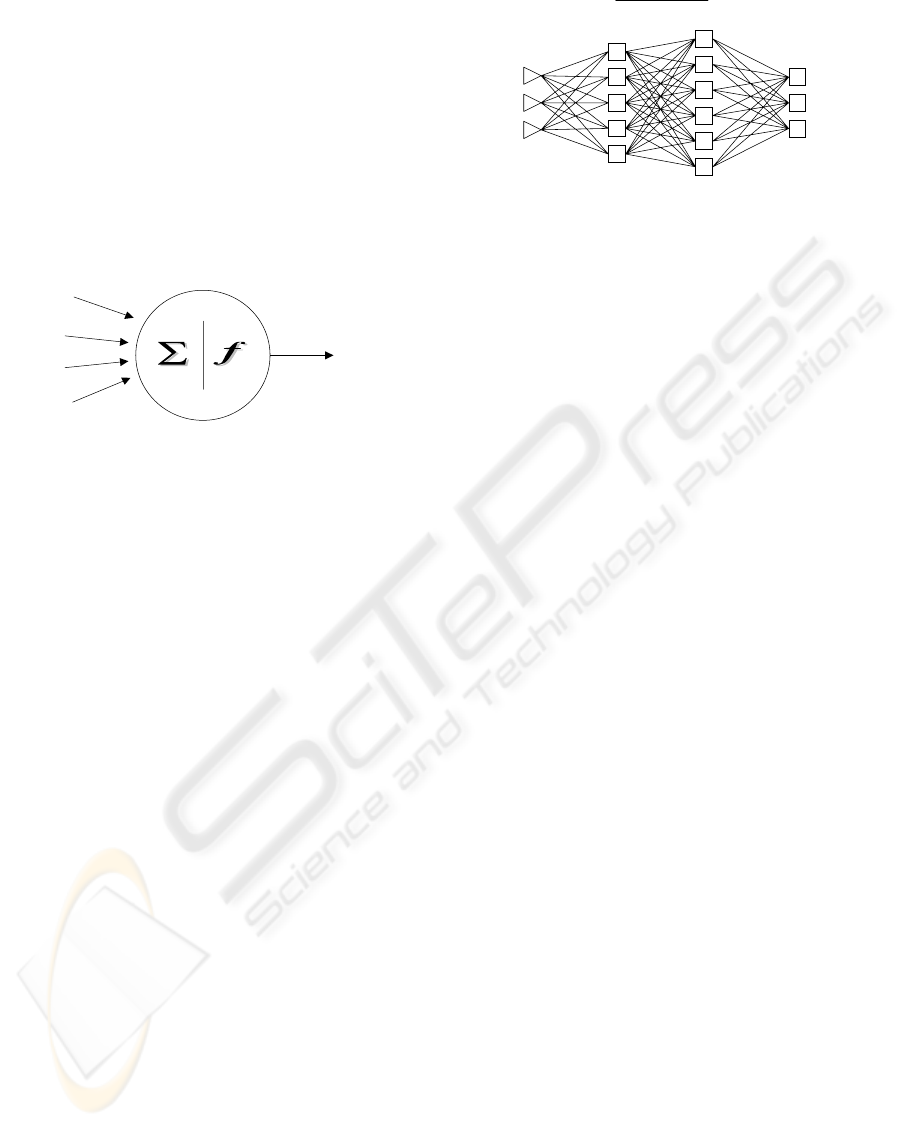
we are trying to solve. Figure 1 represents a picture
of a neuron in a neural network. Each neuron accepts
a weighted set of inputs and responds with an output.
W1
W2
W3
W4
Single Node
Inputs
and
Weights
Summation
and
Activation
Function
Output
Value
Figure 1: A neuron in Neural Network
The real power of neural networks comes when
we combine neurons in multi-layer structures.
Figure 2 represents a sample neural network. The
number of nodes in the input layer corresponds to
the number of inputs and the number of nodes in the
output layer corresponds to the number of outputs
produced by the neural network. When the network
is used, the input variable values are placed in the
input units, and then the hidden and output layer
units are progressively executed. Each of them
calculates its activation value by taking the weighted
sum of the outputs of the units in the preceding
layer, and subtracting the threshold. The activation
value is passed through the activation function to
produce the output of the neuron. When the entire
network has been executed, the outputs of the output
layer act as the output of the entire network.
Once the number of layers and number of units
in each layer has been selected, the network's
weights and thresholds must be set so as to minimize
the prediction error made by the network. This is the
role of the training algorithms. The error of a
particular configuration of the network can be
determined by running all the training cases through
the network, comparing the actual output generated
with the desired or target outputs. The differences
are combined together by an error function to give
the network error.
NEURONS
INPUT LAYER1 LAYER2 OUTPUT
Figure 2: Multi-layer Neural Network
3 SUPPORT VECTOR MACHINES
The support vector machine (SVM) algorithm
(Boser et al., 1992; Vapnik, 1998) is a classification
algorithm that has received a great consideration
because of its astonishing performance in a wide
variety of application domains such as handwriting
recognition, object recognition, speaker
identification, face detection and text categorization
(Cristianini and Shawe-Taylor, 2000). Generally,
SVM is useful for pattern recognition in complex
datasets. It usually solves the classification problem
by learning from examples.
During the past few years, the support vector
machine-learning algorithm has been broadly
applied within the area of bioinformatics. The
algorithm has been used to detect new unknown
patterns within and among biological sequences,
which help to classify genes and patients based on
gene expression, and has recently been used in
several advance biological problems. There are two
main motivations that suggest the use of SVM in
bioinformatics. First, many biological problems
involve high-dimensional, noisy data, and the
difficulty of a learning problem increases
exponentially with dimension. It has been a common
practice to use dimensionality reduction to relief this
problem. SVMs use a different technique, based on
margin maximization, to cope with high dimensional
problems. Empirically, they have been shown to
work in high dimensional spaces with remarkable
performance. In fact, rather than reducing
dimensionality as suggested by Duda and Hart, the
SVM increases the dimension of the feature space.
The SVM computes a simple linear classifier, after
mapping the original problem into a much higher
dimension space using a non-linear kernel function.
In order to control over fitting in this extremely
high-dimensional space, the SVM attempts to
maximize the margin characterized by the distance
between the nearest training point and the separating
discriminant.
Second, in contrast to most machine learning
methods, SVMs can easily handle non-vector inputs,
COMBINING NEURAL NETWORK AND SUPPORT VECTOR MACHINE INTO INTEGRATED APPROACH FOR
BIODATA MINING
183
such as variable length sequences or graphs. These
types of data are common in biology applications,
and often require the engineering of knowledge-
based kernel functions.
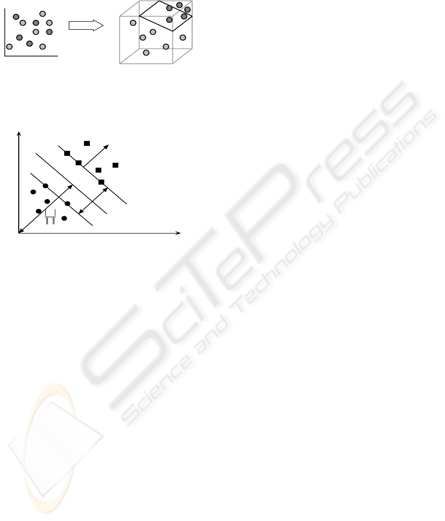
Input Space Feature Space
Φ
Figure 3: Support vector machine: mapping non-
separable data from input space to higher-dimensional
feature space, where a separating hyper-plane can be
constructed.
M
w
Hyperplane
M
1+=+⋅ bxw
T
rr
1−=+⋅ bxw
T
rr
0=+⋅ bxw
T
rr
Margin γ
w
b
r
−
Figure 4: Hyper-plane and margin, circular dots and
square dots represent samples of class -1 and class +1.
4 FEATURE SELECTION
A feature is a meaningful and distinguishing
characteristic of a data sample used by a classifier to
associate it with a particular data category. The
process of selecting or extracting features involves
mathematically manipulating the data sample, and
producing a useful pattern. The process of selecting
or extracting several features to form a feature set is
known as feature selection or feature extraction.
In classification tasks, feature selection is often
used to remove irrelevant and noisy features as well
as producing useful features. The selected feature set
can be refined until the desired classification
performance is achieved. Thus, manually developing
a feature set can be a very time consuming and
costly endeavor. In the area of gene classification by
feature selection, we are interested in identifying the
subset of genes whose expression levels are most
relevant for classification or diagnosis.
In the current bioinformatics research, the
following three approached are mostly considered in
order to do feature selection in gene expression
datasets:
The guiding principle of the first approach is that
the features, which can best be used for classification
of the tissue sample, should be chosen (Xiong et al,
2001). A consequence of this principle is that one
must know exactly how tissue samples will be
classified before feature selection can be done. The
process of feature selection wraps around the
classifier in the following procedure:
(1) A candidate set of features is considered.
a. Tissue samples are divided into training and
test sets.
i. The classifier is trained on the training set of
tissue samples.
ii. The classifier is used on the test set of tissue
samples.
b. Step 1(a) is repeated with alternative divisions
into training and test sets.
c. The candidate feature set is evaluated using all
classifications from 1(a)(ii).
(2) Step 1 is repeated with another candidate feature
set.
In this way, many candidate feature sets are
evaluated using the training set of tissue samples,
and the feature set that performs best is chosen. A
major advantage of the feature wrapper approach is
accuracy, because the feature selection is “tuned” for
the classification method. Another advantage is that
the approach provides some protection against over
fitting because of the internal cross validation. Yet
another advantage will become apparent when
classifiers are employed to distinguish between more
than two tissue types, because most feature selection
methods used to date have been specific to binary
classification. One drawback of feature wrapper
methods is that the methods can be computationally
intensive.
Filter type methods are essentially data pre-
processing or data filtering methods. Features are
selected based on the intrinsic characteristics, which
determine their relevance or discriminant powers
with regard to the targeted classes. In filters, the
characteristics in the feature selection are
uncorrelated to that of the learning methods; thus,
filter methods are independent of the technique for
classifier design; they may be used in conjunction
with any such algorithm, and they have better
generalization property.
In embedded methods, feature selection and
classifier design are accomplished jointly.
Embedded methods incorporate variable selection as
part of the training process and may be more
efficient in several respects: they make better use of
the available data by not needing to split the training
data into a training and validation set; they reach a
solution faster by avoiding retraining a predictor
from scratch for every variable subset investigated.
SVM RFE improves feature selection based on
feature ranking by eliminating the orthogonally
assumptions of correlation methods. This method
ICEIS 2005 - ARTIFICIAL INTELLIGENCE AND DECISION SUPPORT SYSTEMS
184
allows us to find nested subsets of genes that lend
themselves well to a model selection technique that
finds an optimum number of genes. RFE method
uses the following iterative procedure to eliminate
the features:
1. Initialize the data set to contain all features.
2. Train SVM on the data set.
3. Rank features according to criterion c.
4. Eliminate the lowest-ranked feature.
5. If more than one feature remains, return to step
2.
In practice, removing half of the features in step
4 speeds up the algorithm.
RFE ranks the features based on their weight learned
by SVM. Features are re-moved one by one (or by
chunks); SVM is re-run at each iteration.
Among all minimization algorithms for feature
selection using SVMs, RFE has empirically been
observed to achieve the best results on classification
tasks using gene expression data.
5 INTEGRATED APPROACH AND
EXPERIMENTS
For our experiments we used PC with AMD 1900+
CPU, 1GB memory. The experiments were
performed on Matlab 6.5 using Neural Network and
Spider toolboxes.
In our study, we propose and apply the SVM
method of Recursive Feature Elimination (RFE) to
gene selection. By using RFE, we eliminated chunks
of genes at a time. At the first iteration, we reached
the number of genes, which is the closest power of 2.
At subsequent iterations, we eliminated half of the
remaining genes. We thus obtained nested subsets of
genes of increasing informative density. Using
Neural Network as a classifier then assessed the
quality of these subsets of genes. We propose this
method based on the following arguments.
• If it is possible to identify a small set of genes that
is indeed capable of providing complete
discriminatory information, inexpensive diagnostic
assays for only a few genes might be developed
and be widely deployed in clinical settings.
• Knowledge of a small set of diagnostically relevant
genes may provide important insights into the
mechanisms responsible for the disease itself.
• In the cases in which datasets have large number of
features, Neural Networks show their limits on
running time and space complexity. They require
polynomial time and storage space with higher
degree comparing to Support Vector Machines.
And in practice, even 3000-feature-dataset exceeds
the limit of computational power for matrix in
Matlab. Therefore, some approach with lower time
and space complexity like SVM is introduced in
the preprocessing of classification as feature
reduction tool. As a result, we are able to use
Neural Networks to classify datasets that are
generally too big, and cannot be handled by the
Neural Network in their original form.
In the experiment, the general three-layer model
of Neural Network is used as the main classifier.
There are sixty neurons in each layer with their
weights randomly initialized. For the input layer and
hidden layer, the Tan-Sigmoid is chosen as transfer
function, which redistributes input from previous
layer to next layer at the range of [-1, 1]. And the
Log-Sigmoid is used as transfer function on the final
output layer and determines the result --
positive/negative, true/false or class#1/class#0.
Conjugate Gradient Back propagation with Powell-
Beale Restarts (CGB) is the training algorithm for
the network because of its decent performance and
short running-time.
To test our approach we downloaded several
published biological datasets. The datasets used in
the experiments consist of matrix of gene expression
vectors obtained from DNA micro-arrays. We will
provide short description for each dataset.
The first dataset was obtained from cancer
patients with two different types of leukemia. The
problem is to distinguish between two variants of
leukemia (ALL and AML). Distinguishing between
ALL and AML is critical because the two types of
leukemia require different treatment. The dataset
consists of 72 samples (47 ALL vs. 25 AML) over
7129 probes from 6817 human genes.
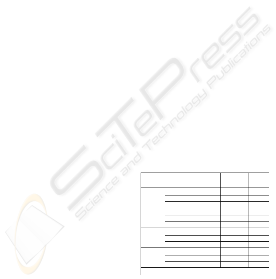
Table 1: Results obtained by using 50/50 ratio for
training data
Highest
Accuracy
Rate
Lowest
Accuracy
Rate
Num
Features
Test vs
Train
(%)
0.9722 0.9444 60 50/50
1 0.9722 50 50/50
ALL/
AML
1 0.9722 40 50/50
0.83 0.60 60 50/50
0.83 0.67 50 50/50
Central
Nervous
System
0.83 0.72 40 50/50
0.9677 0.8710 60 50/50
0.9032 0.7419 50 50/50
Colon
Tumor
0.871 0.7097 40 50/50
0.989 0.956 60 50/50
1 0.989 50 50/50
Lung
Cancer
1 0.9231 40 50/50
Note: Number of Neurons for each NN is 60
COMBINING NEURAL NETWORK AND SUPPORT VECTOR MACHINE INTO INTEGRATED APPROACH FOR
BIODATA MINING
185
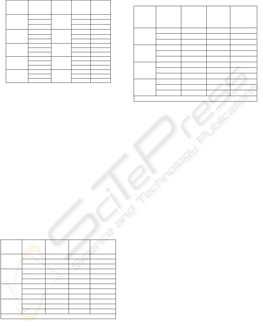
Table 2: Comparison between our method and SVM
Average
Rate
SVM+NN
Average
Rate
SVM
Num
Features
for NN
Train
vs.Test
0.9583 60 50
0.9861 50 50
ALL/
AML
0.9861
0.9361
40 50
0.645
60 50
0.6 50
50
Central
Nervous
S
y
ste
m
0.65
0.6681
40 50
0.72
60 70
0.75
50 70
Central
Nervous
System
0.775
0.6166
40 70
0.80645
60 70
0.7903
50 70
Colon
Tumor
0.8226
0.8080
40 70
0.96155
60 50
0.97255
50 50
Lung
Cancer
0.96155
0.9922
40 50
The purpose of the second datasets is to analyze
the outcome of the treatment. It contains a total of 60
instances. The samples are classified in two classes.
Survivors - patients that responded to the treatment
and Failures – patients that did not benefit from the
treatment. The dataset consists of 21 survivors and
39 failures samples. There are 7129 genes in the
dataset.
The third data set contains 62 samples collected
from colon-cancer patients. Among them, 40 tumor
biopsies are from tumors and 22 biopsies are from
healthy parts of the colons of the same patients. Two
thousand out of around 6500 genes were selected
based on the confidence in the measured expression
levels.
Our fourth data set is used for classification
between malignant pleural mesothelioma (MPM)
and adenocarcinoma (ADCA) of the lung. It consists
of 181 tissue samples (31 MPM vs. 150 ADCA) and
each sample is described by 12533 genes.
Table 3: Results obtained when the training set is 70% of
the data
Highest
Accuracy
Rate
Lowest
Accuracy
Rate
Num
Features
Ratio Test
vs
Train (%)
1 0.9091 60 70/30
1 0.9545 50 70/30
ALL/
AML
1 0.9545 40 70/30
0.76 0.6111 60 70/30
0.7222 0.5556 50 70/30
Central
Nervous
System
0.7222 0.6111 40 70/30
0.95 0.85 60 70/30
0.95 0.80 50 70/30
Colon
Tumor
0.9 0.8 40 70/30
1 0.9815 60 70/30
1 0.8333 50 70/30
Lung
Cancer
1 0.8333 40 70/30
Note: Number of Neurons for each NN is 60
Table 4: Results obtained from increasing the training data
set size to 60% of the data
Highest
Accuracy
Rate
Lowest
Accuracy
Rate
Num
Features
Ratio
Test vs
Train (%)
1 0.9310 60 60/40
1 0.9655 50 60/40
ALL/
AML
1 0.9655 40 60/40
0.7083 0.6667 60 60/40
0.7917 0.6250 50 60/40
Central
Nervous
System
0.72 0.6250 40 60/40
0.9231 0.8077 60 60/40
0.9231 0.8077 50 60/40
Colon
Tumor
0.8846 0.7742 40 60/40
0.9863 0.9231 60 60/40
1 0.9726 50 60/40
Lung
Cancer
0.9863 0.9726 40 60/40
Note: Number of Neurons for each NN is 60
6 THE RESULTS
To normalize the Neural Network training set we
used the formula:
2 ( min( )) /(max( ) min( )) 1normData data data data data
=
×− − −
where normData – normalized value, data – current
value, min(data) – minimum value in the
corresponding column, max(data) – maximum value
in the corresponding column.
The formula normalizes dataset entries in the
range [-1, 1]. Then we mapped the two class
instances to 0 and 1 and then to 0.05/0.95 in order to
use the Log sigmoid transfer function in Neural
Network for the output layer. The initial number of
features for all datasets was too big for the Neural
Network. As a result, we applied the proposed
method and reduced the number of features to 60, 50,
and 40 for the different trials.
In addition, we applied a permutation on the
samples in our datasets. The motivation for such step
was to obtain an even distribution of the two classes
that are going to be classified in both training and
testing sets. Our experiments have shown that if that
condition is not satisfied the performance of the
Neural Network degrades. This was due to the fact
that during the training process the Neural Network
has not seen enough samples from both classes.
To test our network, we divided the datasets in
the training and testing part. The ratios used in
different trials are specified in the results. Finally,
we implemented a program in Matlab that creates 5
different Neural Networks in each trial and outputs
the best results. The accuracy rate that we are
providing is computed as the ratio of the correct
predictions over the total predictions made by the
Neural Network. For example, for ALL/AML
ICEIS 2005 - ARTIFICIAL INTELLIGENCE AND DECISION SUPPORT SYSTEMS
186

dataset using 50/50 ratio for test and train set, the
accuracy rate of 0.9722 that out 36 samples 35 were
correctly classified and only one was predicted
wrong.
7 CONCLUSIONS
As we can see in the results the method we have
proposed in this paper achieves high success rate. In
some trials we obtained a rate as high as 100%. Our
method allows using Neural Networks for a datasets
that are too large in their original form and the
Neural Network is not able to handle the input data.
As a result, we can apply this approach for problems
where it is important to minimize the empirical risk
and the use of a Neural Network is desirable over
SVM classifier.
REFERENCES
Lee Y.-J. and Mangasarian O.L., “RSVM: Reduced
Support Vector Machines,” Proc. SIAM ICDM, 2001.
http://sdmc.lit.org.sg/GEDatasets/Datasets.html
Krishnapuram B., Carin L., and Hartemink A.J., “Joint
Classifier and Feature Optimization for Cancer
Diagnosis Using Gene Expression Data,” Proc. of
RECOMB, 2003.
Weston J., Mukherjee S., Chapelle O., et al, “Feature
Selection for SVMs,” Proc. of NIPS, 2000.
Vapnik V.N., The Nature of Statistical Learning Theory,
Second Ed., Springer, New York, 1999.
Cai C.Z., Wang W.L., Sun L.Z., Chen Y.Z., “Protein
function classification via support vector machine
approach,” Math Biosci., 185(2), pp.111-22, 2003.
Theiler J., Harvey N.R., Brumby S.P., et al, Evolving
Retrieval Algorithms with a Genetic Programming
Scheme, Proc. SPIE 3753, pp.416-425, 1999.
Duda R.O. and Hart P.E., Pattern Classification and Scene
Analysis, John Wiley and Sons, New York, NY, 1973.
Cristianini N., An Introduction to Support Vector
Machines, Cambridge University Press, 2000.
Barzilay and Brailovsky V.L., On domain knowledge and
feature selection using a support vector machines,
Pattern Recognition Letters, Vol.20, No.5, pp. 475-
484, May 1999.
Burgess C., A Tutorial on Support Vector Machines for
Pattern Recognition, Data Mining and Knowledge
Discovery, Vol.2, No.2, pp.121-167, 1998.
Gunn S.R., Support Vector Machines for Classification
and Regression, ISIS technical report, Image Speech
& Intelligent Systems Group, University of
Southampton, 1997
Roth F.P., Bringing Out the Best Features of Expression
Data, Genome Research (Insight/Outlook),
11(11):1801-1802, 2001.
Guyon I., Weston J., Barnhill S., and Vapnik V., “Gene
Selection for Cancer Classification Using Support
Vector Machines,” Machine Learning, Vol.46, Nos.1-
3, pp.389-422, 2002.
Gordon G.J., Jensen R.V., Hsiao L.L., et al, “Translation
of Microarray Data into Clinically Relevant Cancer
Diagnostic Tests Using Gene Expression Ratios in
Lung Cancer and Mesothelioma,” Cancer Research,
62, pp.4963-4967, 2002.
COMBINING NEURAL NETWORK AND SUPPORT VECTOR MACHINE INTO INTEGRATED APPROACH FOR
BIODATA MINING
187
