
FUZZY PATTERN RECOGNITION BASED FAULT DIAGNOSIS
Rafik Bensaadi, Hayet Mouss and Nadia Mouss
Laboratoire d’Automatique et Productique
Université de Batna , 1 Rue Chahid Med. El. Hadi Boukhlouf, 05000 Batna,
Algeria.
Keywords: Diagnosis, fault detection, pattern recognition, fuzzy control, complex plant, conjugate gradients.
Abstract: In order to avoid catastrophic situations when
the dynamics of a physical system (entity in a M.A.S
architecture) are evolving toward an undesirable operating mode, particular and quick safety actions have to
be programmed in the control design. Classic control (PID and even state model based methods) becomes
powerless for complex plants (nonlinear, MIMO and ill-defined systems). A more efficient diagnosis
requires an artificial intelligence approach. We propose in this paper the design of a Fuzzy Pattern
Recognition System (FPRS) that solves, in real time, the main following problems:
Identif
ication of an actual state,
Identif
ication of an eventual evolution towards a failure state,
Diagnosis and decision-making.
1 INTRODUCTION
There is an increasing interest in the development of
intelligent fault detection and diagnosis in industrial
systems because of increasing requirements for
reliable, safe and efficient operation of the plant and
for maintaining quality of the products.
Many variables, unknown or not directly
measured,
have to be included in the state vector to
better describe the plant behaviour: model accuracy,
a very difficult task, is necessary for the effective
processing of unpredictable and imprecise
information. However, human expert can skilfully
control plants, localise a fault and in many times
make a good diagnosis: the human has the ability to
learn, to manage imprecise data and he acts in terms
of a complex combination of sensoring signals
instead of separate information sources. Because of
complexity in modelling a real plant, we need to
achieve this sophisticated level of information
processing that the brain is capable of, to solve the
difficult task of fault detection and diagnosis.
Pattern Recognition is a field concerned with
mach
ine recognition of meaningful regularities in
noisy or complex environments. It is based upon the
numerical representation of the k
th
object observed in
the process (physical entity such as a DC-motor,
photograph, etc.) as a vector x
k
= [x
k1
, . . . ,x
kq
]
T
,
called the pattern vector or feature vector, where x
kj
the j
th
characteristic (feature) associated with
observation k: temperature, pressure, flow, sound
noise frequency, etc. and q the pattern vector length.
Fuzzy logic concept is included to better manage
uncertainty and make useful quantification of hard
attributes.
In this paper, a technique for membership function
app
roximator design is presented. We discuss some
classification approaches and apply CUSUM
algorithm with additional criterions in fault detection
problem. We propose a general diagnosis and
decision making scheme and give simulation results
for a fictive complex system.
2 FPRS DESCRIPTION
The pattern vector corresponds to a combination of
sensoring signals: temperature at point A, pressure
level at B, incoming flow, etc. It is constructed in
terms of the human expert point of view about the
plant, and the effects listed in an FMEA (Failure
Modes and Effects Analysis). Other mathematical
techniques like PCA (Principal Component
Analysis) help to design the pattern vector.
For each new incoming observation, we need to
id
entify and quantify the actual plant status and any
possible convergence toward an other state: in
particular, a failure state. We have to estimate the
347
Bensaadi R., Mouss H. and Mouss N. (2005).
FUZZY PATTERN RECOGNITION BASED FAULT DIAGNOSIS.
In Proceedings of the Seventh International Conference on Enterprise Information Systems, pages 347-356
DOI: 10.5220/0002510403470356
Copyright
c
SciTePress
speed evolution and execute the necessary safety
actions in acceptable delays. A general fault
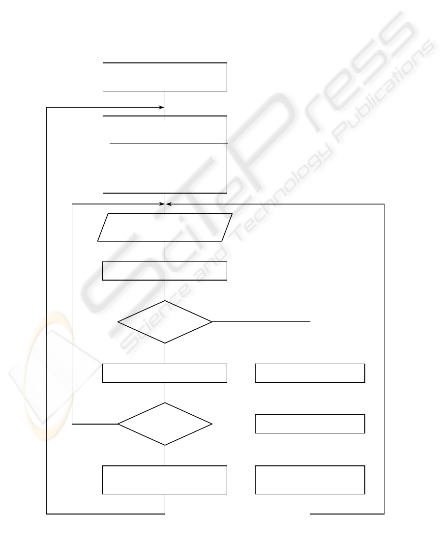
detection and diagnosis that meet these requirements
is presented in figure 1.
3 MEMBERSHIP FUNCTION
ESTIMATION
3.1 Fuzzy Clustering
This first step of unsupervised learning is necessary
to produce a logic initialisation of the fault detection
and diagnosis system.
Given the training set X = {x
1
, x
2
, … x
n
}, where x
k
= [x
k1
, . . . ,x
kq
]
T
the pattern vector, the problem of
fuzzy clustering in X is to assign to the objects {x
k
}
labels that identify ‘natural subgroups’ in X. The
membership degrees, are computed as U = [u
ik
] by
the Fuzzy c-Means (FCM) algorithm with the
following considerations:
A class, set of observations that have similar
properties, corresponds to one operating or
failure mode, the number of clusters c is assumed
to be known. It is also initialised in terms of the
expert point of view,
The training set is considered, as representative
of the whole possible clusters, when its size is
large enough. It is obtained by causing the plant
to operate under different modes.
Initialise c, number of known
operating modes
Membership functions
estimation
Fuzzy Clustering
Training a nonlinear
membership function
approximator
Read z
k
, a new observation,
sequence mean/prototype value
Label z
k
Low
membershi
p
Store as rejected data
Max reached
Update c with a higher
estimation
Classify z
k
State change detection
Monitoring update
Launch safety actions
N
o
Yes
N
o
Yes
Figure 1: A general FPRS design strategy
ICEIS 2005 - ARTIFICIAL INTELLIGENCE AND DECISION SUPPORT SYSTEMS
348

The FCM algorithm converges from any
initialisation to a local minimum. The prototypes
and membership degrees are iteratively updated by
[3]:
∑
∑
=
=
=
n
k
m
ik
q
k
k
m
ik
i
u
u
1
1
x
v
for i = 1,2,…c (1)
u
ik
= f
(x
k
, v
i
, {v
j
}, m)
where,
u
ik
: the membership degree of object x
k
to class i,
v
i
: prototype of class i,
m ∈ [1, ∞): weight exponent on each fuzzy
membership,
until an error threshold is reached.
Expression (1) is intuitively understood when we
observe the similarity with the ‘centre of gravity’
concept.
3.2 Nonlinear Approximator Design
At this step, X = {x
k
} and U = [u
ik
] feed the input of
a nonlinear approximator optimisation algorithm.
Let’s consider the structure of a Radial Basis Neural
Network (RBNN) as shown in figure 2. The hidden
layer is typically comprised of p radial basis
activation functions with an associated Euclidean
input mapping. The output is taken as a linear
activation function with an inner product
Figure 2: RBNN based nonlinear approximator.
The input-output relationship, with x = [x
1
,. . . ,
x
q
]
T
, is given by
∑
=
−−=
p
j
jjj
wF
1
2
2
)/exp(),(
γ
cxθx
(2)
where,
θ = [w
1
, . . . ,w
p
]
T
: the weight vector to be
adjusted during learning,
c
j
= [c
j1
, . . . ,c
jn
]
T
: the centres of Gaussian
functions.
Now, it is desired to cause F
i
(x, θ) to match a
membership function of class i at the data points (x
k
,
{u
ik
}) for i = 1,. . , c, previously estimated by the
FCM. The Conjugate Gradient method, chosen
because of its good convergence properties, is
applied for training the approximator. It is based
upon the minimisation of:
∑
=
=
n
k
kk
i
eeJ
1
T
)(
where,
e
k
= (u
ik
) – F
i
(x
k
, θ), for i = 1,. . . , c
The algorithm is given as follow [10,11]:
1) Calculate
)(
)(
k
i
J
k
θθ
θ
=
∂
∂
=
ζ
. Set the search
direction equal to d(k) = –
ζ
(k).
2) Find θ(k+1) which minimises J
i
(θ) along d(k),
iteratively, by the Secant method:
a) Initialise
σ
< 1, set θ = θ(k)
b) Set
[]
[][]
)()()())((
)()(
TT
T
kdkkdkdk
kdk
ζσζ
ζ
σα
−⋅+
−=
output
c) θ = θ +
α
d(k)
d)
σ
=
α
e) If |
α
⋅d(k)
| < tol
α
then return θ
(k+1) = θ else
go to b
H
idden
layer
3) Calculate
ζ
(k+1).
4) If
θ
ζ
ζ
tol
k
<
)0(
)(
then return θ
(k+1)
x
1
x
q
input
5) Set the next search direction
d
(k+1) = –
ζ
(k+1) +
β
(k+1) d
(k),
where,
[
]
[]
)()(
)1()1(
)1(
T
T
kk
kk
k
ζζ
ζζ
β
++
=+
(Fletcher-Reeves
update), or
FUZZY PATTERN RECOGNITION BASED FAULT DIAGNOSIS
349
[]
[]
)()(
)1()()1(
)1(
T
T
kk
kkk
k
ζζ
ζζζ
β
+−+
=+
(Polak-Ribiere
update)
6) Set k
=
k+1 and goto 2.
c RBNNs are trained to estimate a membership
function for each corresponding class. Note that
F
i
(x, θ) may be outside [0,1] by a very small amount
for the first training, because (2) doesn’t include a
saturation factor. The few false measures must be
corrected (a value that is negative or greater than 1 is
taken, respectively, as 0 or 1) to be processed
correctly for fault detection. An other procedure, that
adds a sigmoid stage to the structure of figure 2, can
be tried in the future.
4 PROCESSING A NEW
OBSERVATION
Once the membership approximator is well defined,
a new observation z is labelled and classified:
The membership value of z to class i is
µ
i
(z) = F
i
(z, θ) (3)
We define a hard classifier on ℜ
q
as a decision
function D imaged in the canonical (unit vector)
basis of Euclidean c-space so that D(z) = e
i
means
that z belongs to class i. This hard attribution is
quantified by (3) to explain how much z is
considered as i
th
fault type and is useful to identify
the actual operating/failure mode. There are many
choices for classifier design:
Criterion 1:
z ∈ i ⇔ µ
i
(z) = max {
µ
j
(z)
}
j = 1, ⋅⋅⋅ c
. (4)
Criterion 2
: crisp nearest prototype rule (NP rule)
z ∈ i ⇔ D
NP,v
(z) = e
i
⇔ || z – v
i
|| ≤ || z – v
j
||
for j = 1, ⋅⋅⋅ c. (5)
Criterion 3
: fuzzy k-nearest neighbor (k-NN) rule
Compute and rank the distances d(z, x
i
) as {d
1
≤ d
2
≤
⋅⋅⋅ d
k
≤ d
k+1
≤ ⋅⋅⋅ d
n
}. Find the columns in U
corresponding to the k nearest neighbor indices {1,
2, ⋅⋅⋅ k}. Calculate the vector u(*|z) = [u(1|z) u(2|z)
⋅⋅⋅ u(c|z)]
T
with the NN labels:
∑
=
=
k
j
ij
k
u
iu
1
) ( z for j =
1, ⋅⋅⋅ c.
And finally decide
z ∈ i ⇔ D
NN,k
(z) = e
i
⇔ u(i|z) = max {
u(j|z)
}
j = 1, ⋅⋅⋅ c
.
(6)
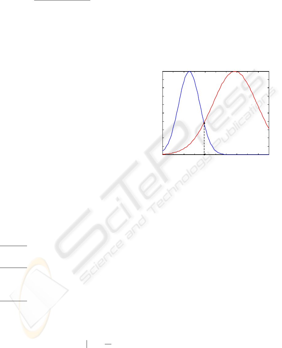
For a long training set and an efficient
approximator, the first criterion is the most adequate.
NP and k-NN may be used as a redundant alternative
to solve ambiguous situations like the example
illustrated in figure 3: it is easy to see that (z
1
<z* ∈
class 1) and (z
2
>z*∈ class 1), but we need an
additional/other criterion to classify (z
2
≈ z*)
0 0.1 0.2 0.3 0.4 0.5
0.6
0.7
0.8
0.9 1
0
0.1
0.2
0.3
0.4
0.5
0.6
0.7
0.8
0.9
1
z
membership function
µ1(z)
µ2(z)
z
*
Figure 3: Example of an ambiguous classification
problem
.
We add the constraint
th
c
i
i
uµ >
∑
=1
)(z
(7)
to reject observations with low membership degrees,
u
th
is a small nonzero number taken lower than 0.5.
When a sufficient number of similar (low variance
for a Gaussian pdf approximation) observations are
reached, a new cluster is created. Prototype and
membership function parameters are computed
individually (partial FCM with c=1) or by restarting
a global membership function estimation process.
5 FAULT DETECTION AND
FORECASTS
This is a more ambitious and potentially useful task
in maintenance monitoring. The detection of an
actual or future operating/failure mode requires
getting and processing, in real time, the signals z(t)
and µ
i
(z,t), and taking advantage of their stochastic
properties. If the plant status is efficiently described
by the pattern vector, we note by µ
i
(t) the
membership degree of the plant state to class i at
ICEIS 2005 - ARTIFICIAL INTELLIGENCE AND DECISION SUPPORT SYSTEMS
350

time t, and we develop our approach through the
following steps:
1) CUmulative SUM (CUSUM) algorithm is
involved in change detection by processing a
sequence of independent random variables with
probability density function p
Θ
(z) depending
upon one parameter Θ. It relies on a fundamental
concept: the log-likelihood ratio of an
observation z:
)(
)(
ln)(
0
1
z
z
z
Θ
Θ
=
p
p
s (8)
before an unknown change time k
0
, Θ is equal to
Θ
0
. At time k
0
, it changes to Θ = Θ
1
≠ Θ
0
. The
problem is to detect the change time.
The cumulative sum
∑∑
=
Θ
Θ
=
==
k
j
k
j
jp
jp
jskS
1
0
1
1
))((
))((
ln))(()(
z
z
z
(9)
(where, {z(j)}
j = 1, ⋅⋅⋅ k
a sequence of independent
random variables) is expected to exhibit a
negative drift before change, and a positive drift
after change. CUSUM algorithm is derived under
this idea and given as follow:
At each sample time,
a) Acquire the new data z(k),
b) Compute the decision function
g(k)=max{0, g(k-1)+s(z(k))},
c) Compute the number of successive
observations for which the decision function
remains strictly positive:
N(k) = N(k-1) 1
{g(k-1)>0}
+1,
where 1
{x}
=1 when x is true and 1
{x}
= 0
otherwise.
d) If g(k) > h, issue an alarm, (h is a threshold
chosen to meet either a specified mean time
for detection or a specified mean time
between false alarms)
Find the change occurrence time: k
0
= k
a
–
N(k
a
), where k
a
is the alarm time,
Reinitialise the decision function to 0,
In many practical cases, Θ is taken as the mean
value of a Gaussian distribution p
Θ
(z). In our
problem, each typical value Θ
i
indicates a class
prototype v
i
, and the problem of change
detection between failure modes will require a
prior knowledge about the class-statistical
properties. We only own a membership function
database!
2) Because of the fact stated above, CUSUM will
be applied with the following modification:
)(
)(
ln
z
z
j
i
µ
µ
is considered instead of
)(
)(
ln
z
z
j
i
p
p
Θ
Θ
where i and j are class-indexes. A membership
value doesn’t have the same meaning as
probability, but the ratios reflect the same
information, so the ability to apply CUSUM with
taking
)(
)(
ln)(
z
z
z
j
i
µ
µ
s =
(10)
is intuitively concluded.
3) Change time detection between two states is
presented. If the target class prototype remains
far, k
0
may be considered as an evolution
detection occurrence and safety decisions are
executed in acceptable delay. When the radius of
target class membership function is very small,
the safety task will be more difficult, so we need
an other tool to better quantify the evolution
between states and make an earlier alarm.
An evolution towards a fault is described by
dt
td
i
)(
µ
: A negative value means that the plant is
leaving state i, a positive value means that it is
evolving towards this state. The evolution speed
attributes ‘quick’ or ‘slow’ are quantified by
2
2
)(
dt
td
i
µ
: the change in evolution speed is said to
be ‘quick’ for
0
)(
2
2
>
dt
td
i
µ
, an observation may
leave quickly state i while converging slowly to
state j. Information about the fault evolution
direction are extracted from a 3×c matrix defined
by:
⎥
⎥
⎥
⎥
⎥
⎥
⎥
⎦
⎤
⎢
⎢
⎢
⎢
⎢
⎢
⎢
⎣
⎡
=
2
2
2
2
2
2
1
2
21
21
...
...
...
E
dt
µd
dt
µd
dt
µd
dt
dµ
dt
dµ
dt
dµ
µµµ
c
c
c
(11)
The corresponding alarme time k
e
is computed
in terms of constraints on the elements of E. For
example, k
e
may be defined as the delay time for
which both
⎟
⎠
⎞
⎜
⎝
⎛
dt
td
i
)(
µ
and
⎟
⎟
⎠
⎞
⎜
⎜
⎝
⎛
⋅
2
2
)()(
dt
td
dt
td
ii
µµ
FUZZY PATTERN RECOGNITION BASED FAULT DIAGNOSIS
351

remain positive, and this corresponds to the
alarm time k
a
computed by CUSUM. Other
conditions may be added to make an earlier
alarm (optimisation problem).
Because of external disturbances, a noise is
added to z when reading. We’ll consider mean
values instead of instantaneous values: the
problem is solved by a digital FIR filter, the
frequency bandwidth and sampling time are
chosen in terms of the noise properties and the
response time of all the mechanical/electrical
plant parts considered in the diagnosis design.
6 DIAGNOSIS AND DECISION
MAKING
We completely described a fault detection scheme.
The i
th
fault type effects (symptoms) may be caused
by more than one physical entity, and this fact is
described by conditional probabilities. Diagnosis is
to decide that element e
j
(a valve, transistor, heater,
etc) is (or will be) the cause of the detected (or
expected) fault. Previous fault events feed a
statistical database with class-conditional pdf(s)
{p(i
th
fault | e
j
-fault)}, used to compute p(e
j
-fault | i
th
fault) by Bayes’ rule. The corresponding safety
actions are made according to the diagnosis
conclusion, the fault severity and the decision
making scheme. One powerful solution is built upon
an Inference Engine: this is a software or hardware
system, which gives a conclusion (output) from a
fact (input) and knowledges (production rules). If
knowledges include fuzzy linguistic terms, it is
referred to as Fuzzy Inference Engine (FIE).
A conclusion may deal with:
• A new reference tracking (fuzzy control), the
knowledge base includes rules of the form:
if (mode2) and (low inflow), then (tank 3
temperature should be low)
• Diagnosis / binary logic instructions, a production
rule may be:
if (water outflow > 0.24m
3
/s) and (valve 21
closed), then (shut-off and repair/change element
e
2
),
if (d
2
µ
3
/dt
2
>0.12) or (input control u
1
not set), then
(3
rd
fault type in the next 3 minutes).
Beyond the construction/generation of production
rules, one difficult task when implementing a fuzzy
control algorithm is the accuracy of meaningful
membership functions for all the fuzzy linguistic
terms considered in the knowledge base. We’ll
present later, through an example of temperature
control, the different steps involved in fuzzy control
implementation.
7 SIMULATION RESULTS
For the demonstration of the proposed diagnosis
method, we consider a fictive complex process. We
assumed that a human expert was supervising the
plant state by observing three variables: v
1
(pressure
at point A
1
), v
2
(temperature at point A
2
) and v
3
(sound noise frequency). He makes detection and
diagnosis upon two complex combinations: x
1
=f
1
(v
1
,
v
2
, v
3
) and x
2
= f
2
(v
1
, v
2
, v
3
) (PCA). We want to apply
the designed FPRS to act with a similar reasoning
faculty.
Simulation is run, by causing the plant to operate
during a sufficient time, under one normal (typical)
operating mode and two failure modes (plant
parameters randomly affected). PCA has reduced the
pattern vector to [x
1
, x
2
]
T
. The unsupervised learning
step is applied with a training set of 100 data points.
Samples are labelled; and the prototypes identified
as shown in figure 4.
-2 0 2 4 6 8 10 12
-6
-4
-2
0
2
4
6
8
x1
x2
Figure 4: Fuzzy clustering with c=3, q=2. The prototypes
are marked as red stars: v
1
=[1.823, -0.935]
T
, v
2
=[9.006,
2.151]
T
, v
3
=[6.297, 5.078]
T
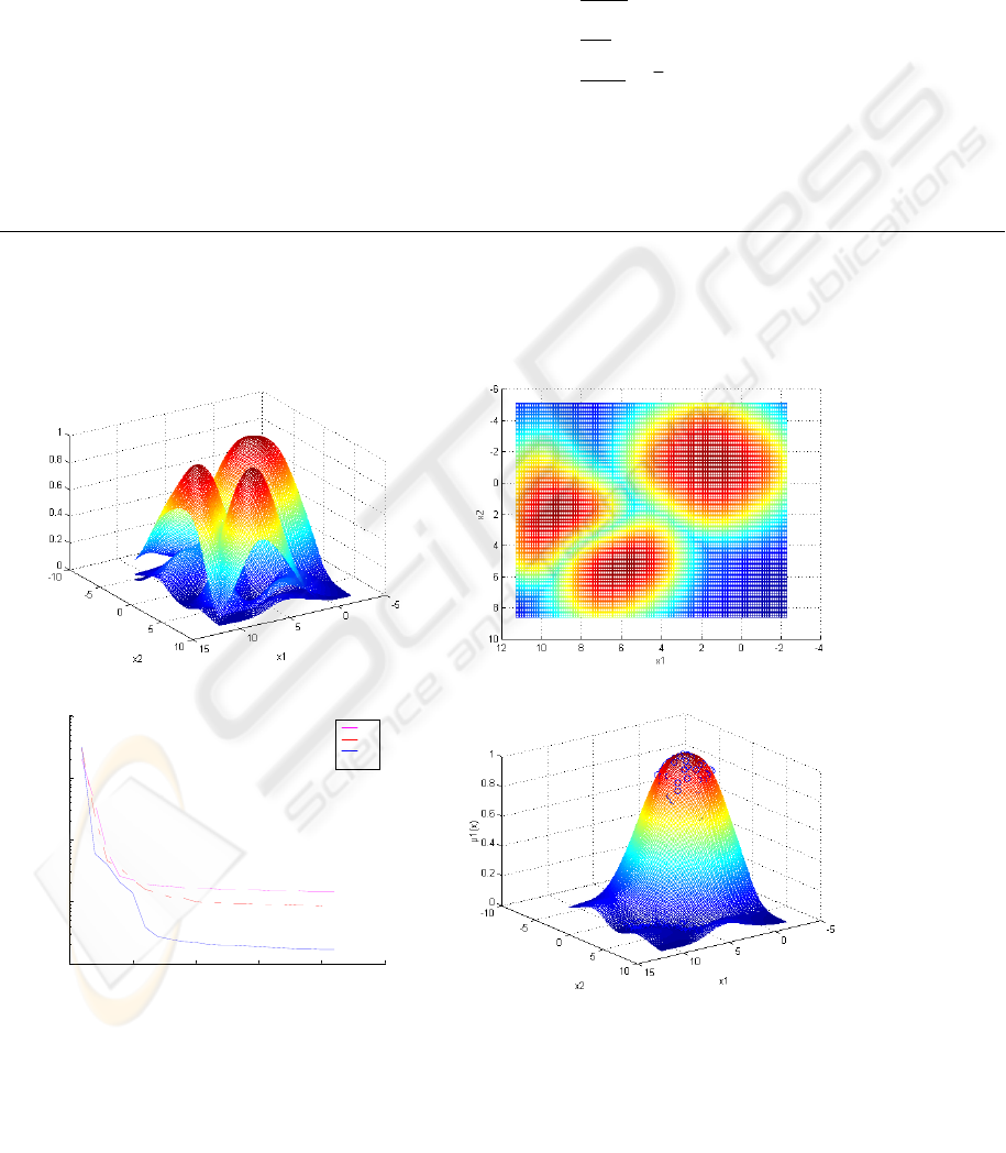
The method of Conjugate Gradients is successfully
applied to train an RBNN based membership
function approximator for each class (figure 5).
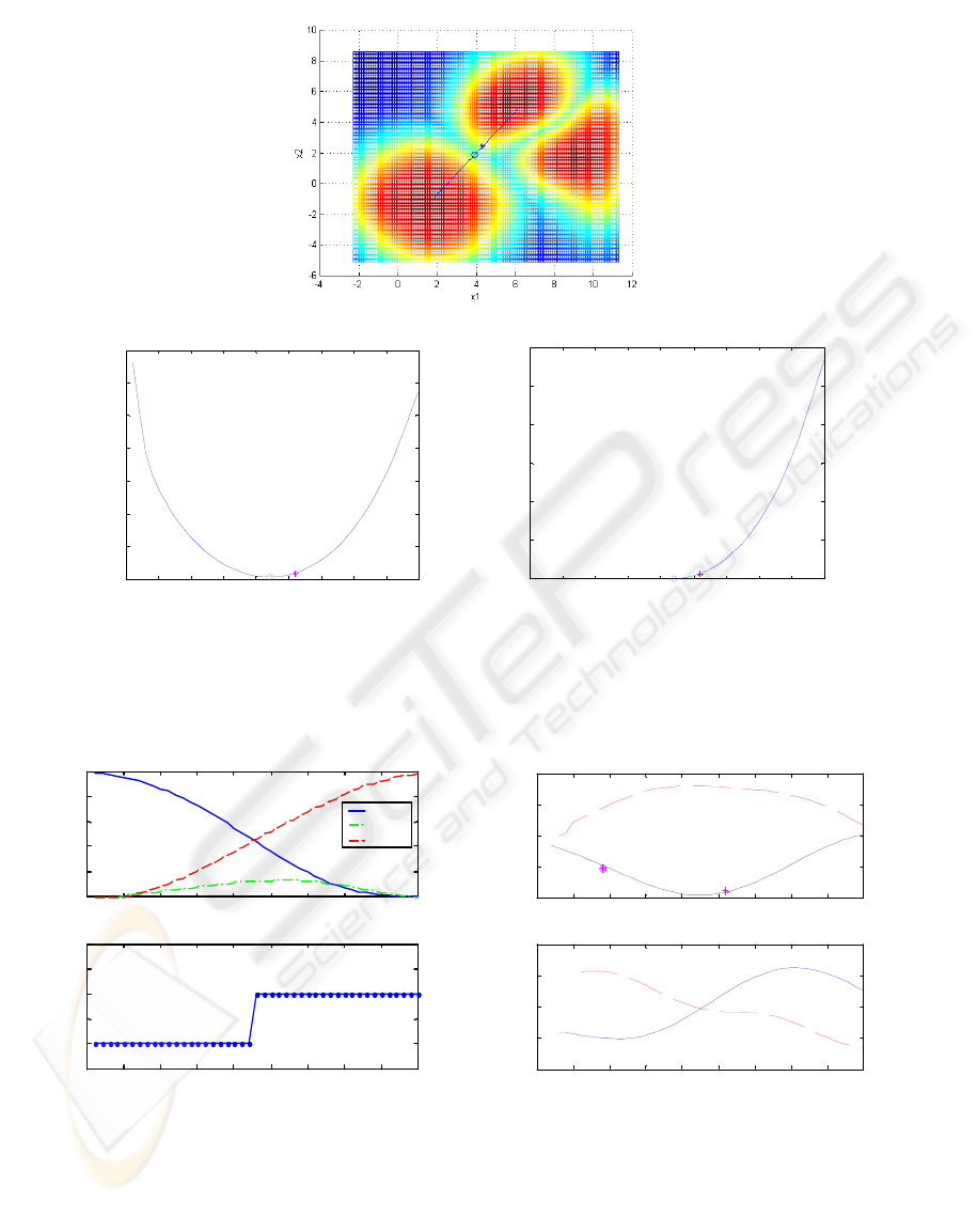
For classification and fault detection test, we
caused the system to evolve towards mode 3 by
generating a linear path sequence {z
k
=[z
k1
, z
k2
]
T
},
each observation is well labelled and classified
(Figure9-a). CUSUM is applied with
)(
)(
ln)(
1
3
z
z
z
µ
µ
s =
(figure 6). Evolution towards fault 3 is detected
ICEIS 2005 - ARTIFICIAL INTELLIGENCE AND DECISION SUPPORT SYSTEMS
352
The fuzzy linguistic term ‘mode i’ is described by
the corresponding membership function F
i
(x,θ). The
membership function for each other fuzzy linguistic
term is initialised as shown but may be modified by
learning to update the shape form and parameters.
earlier when membership function derivatives are
considered (figure 7-b).
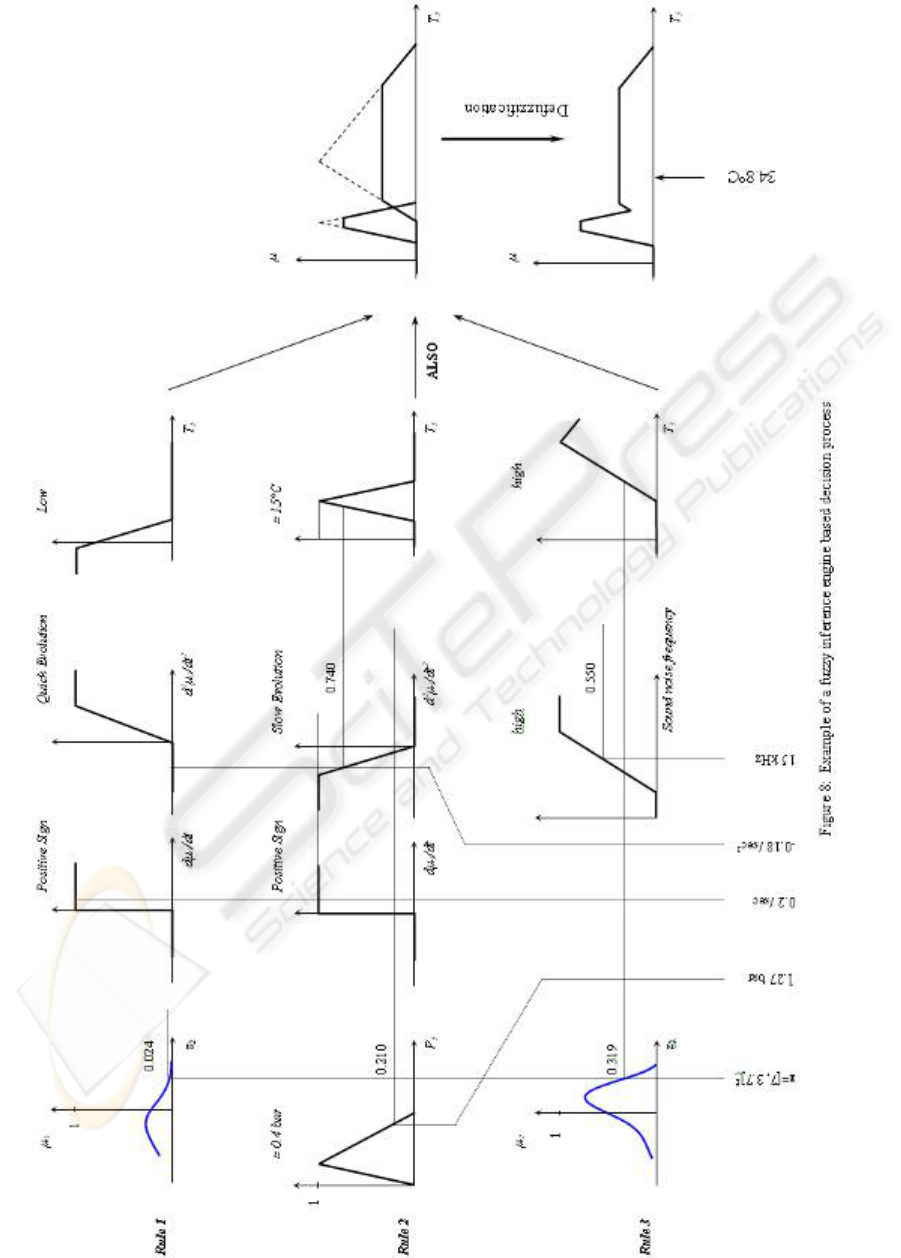
Temperature control problem is presented to
describe an exemple of a fuzzy inference engine
(figure 8). A part of the knowledge base is given as
follow:
The basic operators, involved in fuzzy control, are
defined as follow:
R1: if (mode1) and (quick evolution toward mode3),
then (T
5
should be low)
R2: if (P5 ≈ 0.4 bar) or (slow evolution toward mode3)
, then (T
5
should be around 15°C)
R3: if (mode2) and (high sound noise frequency),
then (T
5
should be high)
…..
Fact: z=[7, 3.7]
T
, P
5
= 1.27 bar, dµ
3
/dt
= 0.2 /sec, d
2
µ
3
/dt
2
= -0.18 /sec
2
, f
sn
= 15 kHz
Conclusion: T
5
should be ?
AND
: µ
A∩B
=
MIN(µ
A
, µ
B
) (12)
OR
: µ
A∪B
=
MAX(µ
A
, µ
B
) (13)
NOT
:
A
A
1
µ
µ
−
=
(14)
(a) (b)
0 5 10 15 20 25
10
-2
10
-1
10
0
10
1
10
2
number of iterations
J3
J2
J1
(c) (d)
Figure 5: membership approximator, p=25, γ = 2.5. (a) Plant status membership functions. (b) Projection of (a) on
x
1
-x
2
plane, the similarity with the plot of figure 4 is proved. (c) Cost function during learning. There is a trade-off
between the learning time and accuracy requirements. (d) F
1
(x, θ) matches the data pairs considered in training the
RBNN
.
FUZZY PATTERN RECOGNITION BASED FAULT DIAGNOSIS
353
(a)
0 5 10 15 20 25 30 35 40 45
-80
-70
-60
-50
-40
-30
-20
-10
time in number of samples
CUmulative SUM: S
(b)
0 5 10 15 20 25 30 35 40 45
0
10
20
30
40
50
60
time in number of samples
cusum decision function: g
(c)
Figure 6: Fault change detection by CUSUM, h=1.2. The estimated change occurrence is marked as circle; the alarm
time as star. (a) New observation-path, plant is leaving mode1 towards mode3 (b) Cumulative Sum plot, (c) decision
function plot
.
0
5
10
15
20
25
30
35
40
45
0
0.2
0.4
0.6
0.8
1
time in number of samples
Membership
µ1(z(k))
µ2(z(k))
µ3(z(k))
0
5
10
15
20
25
30
35
40
45
0
1
2
3
4
5
time in number of samples
Class number
(a)
0 5 10 15 20 25 30 35 40 45
-0.04
-0.02
0
0.02
0.04
time in number of samples
membership first derivative
0 5 10 15 20 25 30 35 40 45
-4
-2
0
2
4
x 10
-3
time in number of samples
membership second derivative
(b)
Figure 7: Future fault detection strategy with additional derivative based criterions. (a) Criterion 1-classification. (b)
1
st
and 2
nd
derivatives of µ
1
(t) and µ
3
(t), the filled circle indicates an earlier change detection.
ICEIS 2005 - ARTIFICIAL INTELLIGENCE AND DECISION SUPPORT SYSTEMS
354
FUZZY PATTERN RECOGNITION BASED FAULT DIAGNOSIS
355

For each rule, the compatibility of the fact to the
antecedent is obtained by projecting the fact to the
corresponding membership function. The resulting
membership degrees are combined by a conjunction
‘AND’ (rules 1, 3) or ‘OR’ (rule 2). An individual
conclusion is obtained by truncating (minimising)
the consequent membership function. All the rules
are combined by conjunction ‘ALSO’ (maximisation
of individual conclusions) to construct a relatively
complicated membership function ‘µ’ characterising
the final conclusion. The final step is
defuzzification: the new reference
that must be
tracked, given the fact: (z=[7, 3.7]
T
, P
5
=1.27 bar,
dµ
3
/dt = 0.2 /sec, d
2
µ
3
/dt
2
=-0.18 /sec
2
, f
sn
=15 kHz),
is computed by the center-of-gravity method:
*
5
T
()
()
C8.34
55
555
*
5
°==
∫
∫
dTTµ
dTTµT
T
(15)
and T
5
remains continuously under this control.
8 CONCLUSION
We have proposed a general FPRS design scheme
for fault detection and diagnosis in industrial
systems. This approach involves fuzzy clustering as
a first partition of the training set into a number of
classes initialised by the known operating/failure
modes, and the conjugate gradient method as the
learning tool for training membership function
approximators. Incoming observations will be
classified and new created classes are taken into
account.
Fault detection efficiency is first tested by
applying CUSUM with modified expression of the
log-likelihood ratio: membership degrees are
considered instead of probabilities. Then, an other
proposed method that takes advantage of
membership function derivatives is investigated,
evolution towards a fault type target is quantified
and safety actions will be executed in acceptable
delays.
There are many ways to design the decision
system, we proposed a knowledge based approach
and presented a ‘temperature fuzzy control’ as an
example of a safety action based on information
about fault change forecasts, extracted from the
matrix E.
The designed FPRS is successfully tested for a
fictive plant. Its proficiency will be more proven
when tested in a real environnement, this involves
additional hardware and software implementation
and will be the subject of a future work.
REFERENCES
Mogens Blanke, Michel Kinnaert, Jan Lunze and Marcel
Staroswiecki, 2003. Diagnosis and fault tolerant
control, Berlin: Springer.
L. H. Chiang, E .L. Russell and R. D. Braatz, Fault 2001.
Detection and Diagnosis in Industrial Systems,
London: Springer.
J. C. Bezdek, 1996. a review of probabilistic, fuzzy, and
neural models for pattern recognition. In C. H. Chen
(ed), Fuzzy logic and neural network handbook,
chapter 2, New York: McGraw Hill.
L. A. Zadeh, 1965. Fuzzy sets. Information and Control,
vol. 8, pp. 338-353.
L. A. Zadeh, 1973. Outline of a new approach to the
analysis of complex systems and decision processes’,
IEEE Trans. Syst., Man, Cybern., vol. SMC-3, no. 1,
pp. 28-44, jan.
S. Zieba, 1995. Une méthode de suivi d’un système
évolutif. Application au diagnostic de la qualité
d’usinage, Thèse de doctorat, Université de
Technologie de Compiègne, juin.
Takeshi Yamakawa 1993. A Fuzzy Inference Engine in
Nonlinear Analog Mode and Its Application to a
Fuzzy Logic Control. IEEE trans. on Neural
Networks, vol. 4, no. 3, pp. 496-522, May.
I. S. Torsum, , 1995 Foundations of Intelligent
Knowledge-Based Systems, London: Academic Press.
Bernard Dubuisson, Diagnostic et reconnaissance des
formes, Paris: Hermès, 1990.
Jonathan Richard Shewchuk, 1994. An Introduction to the
Conjugate Gradient Method Without the Agonizing
Pain (e-article), August.
Jeffrey T. Spooner, Manfredi Maggiore, Raúl Ordóñez and
Kevin M. Passino, Stable 1996. Adaptive Control and
Estimation for Nonlinear Systems. –Neural and Fuzzy
Approximator Techniques, New York: John Wiley and
sons, Inc.
David J. DeFatta, Joseph G. Lucas and William S.
Hodgkiss, 1988. Digital Signal Processing: A System
Design Approach, New York: John Wiley and sons,
Inc.
ICEIS 2005 - ARTIFICIAL INTELLIGENCE AND DECISION SUPPORT SYSTEMS
356
