CLUSTERING INTERESTINGNESS MEASURES WITH POSITIVE

CORRELATION

Xuan-Hiep Huynh, Fabrice Guillet, Henri Briand

LINA CNRS FRE 2729 - Polytechnic school of Nantes university

La Chantrerie BP 50609 44306 Nantes Cedex 3, France

Keywords:

Interestingness measure, intensity of implication, cluster, objective measure, interestingness property.

Abstract:

Selecting interestingness measures has been an important problem in knowledge discovery in database. A lot

of measures have been proposed to extract the knowledge from large databases and many authors have intro-

duced the interestingness properties for selecting a suitable measure for a given application. Some measures

are adequate for some applications but the others are not, and it is difﬁcult to capture what the best measures

for a given data set are. In this paper, we present a new approach implemented in a tool to select the groups or

clusters of objective interestingness measures that are highly correlated in an application. The ﬁnal goal relies

on helping the user to select the subset of measures that is the best adapted to discover the best rules according

to his/her preferences.

1 INTRODUCTION

Many interestingness measures have been proposed

in the literature to select the most signiﬁcant knowl-

edge from a large database in knowledge discovery in

database research such as support, conﬁdence, causal

support, laplace, lift, cosine, gini-index, conviction,

loevinger, yule’s y, intensity of implication entropy’s

version, ... in order to reduce the enormous amount

of rules discovered under the form of association rules

introduced by Agrawal (Agrawal et al., 1993). Each

measure is used with its own characteristics of a given

domain of application so that it is not adequate for a

given domain of application that is strongly different.

There are two types of measures (Freitas, 1999): sub-

jective and objective. Subjective measures (Padman-

abhan and Tuzhilin, 1998) (Liu et al., 1999) depend

on the user who examines the data with his/her ex-

periences while objective measures depend only on

the data structure. The problem of ﬁnding interesting

patterns leads to the design of a suitable measure and

the deﬁnition of a set of principles or properties (Sil-

berschartz and Tuzhilin, 1996)(Gavrilov et al., 2000)

(Klemettinen et al., 1994) (Brin et al., 1997) (Bayardo

and Agrawal, 1999) (Hilderman and Hamilton, 2001)

(Tan et al., 2004). In our works, we focus on the ob-

jective interestingness measures.

The paper is organized as follows. Section 2

gives the deﬁnition and approach with the concepts

of intensity of implication. Section 3 introduces an

overview of interestingness properties proposed in the

literature and determines some mathematical relation

of the measures. Section 4 presents our approach on

cluster analysis. Section 5 gives the ﬁrst results of our

works in ﬁnding the clusters of interestingness mea-

sures. Finally, we conclude and introduce some future

research works.

2 INTENSITY OF IMPLICATION

Gras (Gras, 1996) introduced the theory of statisti-

cal implication, with the concepts of examples and

negative examples (contra-example). We consider the

quality of the implication and determine this quality

with the change of negative examples.

An association rule a ⇒ b is an implication that b

tends to be true once we know a. But it is difﬁcult to

see this case in reality. There is always some nega-

tive examples that b is false when a is true. Intensity

of implication (Gras, 1996) is a measure ϕ(a ⇒ b)

based on the probability model of association rule and

giving the user some thing interesting by considering

the effects of the number of negative examples on the

decision. Intensity of implication is also a robustness

approach for the evaluation of the data set by just tak-

248

Huynh X., Guillet F. and Briand H. (2005).

CLUSTERING INTERESTINGNESS MEASURES WITH POSITIVE CORRELATION.

In Proceedings of the Seventh International Conference on Enterprise Information Systems, pages 248-253

DOI: 10.5220/0002508502480253

 SciTePress

ing in account a small number of negative examples.

Each association rule a ⇒ b must be associated to 4

cardinalities (n, n

, n

). More precisely, n is the

number of transactions, n

(resp. n

) the number of

transactions satisfying the itemset a (resp. b), and n

is the number of transactions satisfying a∧

b (negative

examples).

Figure 1: Cardinalities of a rule a ⇒ b.

With these notions, p(a), p(b), p(a∧b), p(a∧b) are

the probabilities of the premise, conclusion, negative

examples, and examples of the rule respectively com-

puted as:

With all the studied interestingness measures, we

are going to calculate as one function f with four

arguments n, n

, n

. Then, all the quality mea-

sures will be transformed in terms of n, n

, n

, and

. See Appendix A.

3 INTERESTINGNESS

PROPERTIES

Objective measure is a data-driven, domain-

independent approach to evaluate the quality of

discovered patterns. Piatetsky-Shapiro (Piatetsky-

Shapiro, 1991) proposed three principles for a

suitable rule-interest measure (RI) on a rule a ⇒ b:

(P1) RI = 0 if a and b are statistically independent;

the rule is not interesting, (P2) RI monotonically

increases with p(a ∧ b) when p(a) and p(b) remain

the same, (P3) RI monotonically decreases with p (a)

or p(b) when the rest of the parameters (p(a ∧ b) and

p(b) or p(a)) remain unchanged.

There are many authors who have extended these

principles or proposed new principles:

(Bayardo and Agrawal, 1999) concluded that the

best rules according to any interestingness measures

must reside along a support/conﬁdence border. The

work allows for improved insight into the data and

supports more user-interaction in the optimized rule-

mining process.

(Hilderman and Hamilton, 2001) proposed ﬁve

principles for ranking summaries generated from

databases, and performed a comparative analysis of

sixteen diversity measures to determine which ones

satisfy the proposed principles. The objective of this

work is to gain some insight into the behavior that can

be expected from each of the measures in practice.

(Kononenco, 1995) analyses the biases of eleven

measures for estimating the quality of multi-valued

attributes. The values of information gain, j-measure,

gini-index, and relevance tend to linearly increase

with the number of values of an attribute.

(Tan et al., 2004) introduced twenty-one interest-

ingness measures using Pearson’s correlation and has

found two situations in which the measures may be-

come consistent with each other, namely, the support-

based pruning or table standardization are used. In

addition, he also proposed ﬁve new interestingness

properties: (1) symmetry under variable permutation,

(2) row/column scaling invariance, (3) anti-symmetry

under row/column permutation, (4) inversion invari-

ance, and (5) null invariance, to capture the utility

of an objective measure in terms of analyzing k-way

contingency tables.

Our approach is different because we consider the

data set values with the intensity of implication mea-

sure, taking into account the number of negative ex-

amples in the data sets, while the other authors have

investigated the properties of interestingness on the

basis of their own approaches, not on the data set.

Furthermore, we have found some relations in

mathematical formulae of the quality measures. This

work is useful and interesting for reducing the quan-

tity of measures. If one measure strongly depends on

the other measures, we will not consider it any more.

For example: T auxDeLiaison = Lift − 1, we will

only select Lift for both of them. See Appendix B.

4 CLUSTER ANALYSIS

4.1 Correlation

We extended the deﬁnition of similarity between two

associations patterns introduced by Tan (Tan et al.,

2004):

Let R(D) = {r

, r

, ..., r

} denote input data as

a set of p association rules derived from a data set

D. Each rule a ⇒ b is described by its itemsets

(a, b) and its cardinalities (n, n

, n

). Let M

be the set of q available measures for our analysis

M = {m

, m

, ..., m

}. Each measure is a numer-

ical function on rule cardinalities: m(a ⇒ b) =

f(n, n

, n

For each measure m

∈ M , we can construct a vec-

tor m

(R) = {m

, m

, ..., m

}, i = 1..q, where

corresponds to the calculated value of the mea-

sure m

for a given rule r

The correlation value between any two measures

, m

{i, j = 1..q} on the set of rules R will be cal-

culated by using a Pearson’s correlation coefﬁcient

CLUSTERING INTERESTINGNESS MEASURES WITH POSITIVE CORREALTION

249

CC (Saporta, 1990), where m

, m

are the average

calculated values of vector m

(R) and m

(R) respec-

tively.

CC(m

, m

) =

k=1

[(m

−

)(m

− m

)]

[

k=1

−

)

][

k=1

− m

)

]

Deﬁnition 1. Strongly positive/negative correlated

measures. Two measures m

and m

are strongly pos-

itive (resp. negative) correlated to each other with re-

spect to the data set D if the correlation value between

and m

is greater (resp. lower) than or equal to a

threshold t

(resp. t

Deﬁnition 2. Uncorrelated measures. Two mea-

sures m

and m

are uncorrelated to each other with

respect to the data set D if the absolute value of the

correlation between them is lower than or equal to a

critical value t

In our experiment, we use t

= 0.85, t

= −0.85,

and t

= 1.960 ×

√

(a level of signiﬁcance of the

test α = 0.05 for hypothesis testing) in a population

p because of their wide acceptation in the literature.

Deﬁnition 3. Positively correlated cluster. A con-

nected component of the graph that is based on the

similarity matrix in which each strongly positive cor-

relation between two measures represents an edge, it

is a positively correlated cluster.

4.2 A quick description of data and

measures used

We have applied our experiments on the rule set of

120000 association rules. The rules have been ex-

tracted from the ”Mushroom” data set by using the

Apriori algorithm (Agrawal and Srikant, 1994). The

Mushroom data set is issued from one of the categor-

ical data set from Irvine machine-learning database

repository (Blake and Merz, 1998).

In our experiment, we compared and analyzed 34

interestingness measures (see Appendix A for com-

plete deﬁnitions).

As announced, we will present some interesting re-

sults of the Mushroom data set, focusing on cluster

results.

5 FIRST RESULTS ON CLUSTER

ANALYSIS

5.1 Distributions

Frequent and inverse-cumulative histograms are in-

troduced to present the frequency of values calcu-

lated from the measures in one cluster. The minimum,

maximum, average, skewness and kurtosis values are

computed in order to allow the user to have a ﬁrst view

of all the measures in the cluster (Fig. 2).

Figure 2: Distribution of one cluster from Mushroom data

set.

We have determined all the scatter plots that can be

generated from every pair of measures, and it takes

a lot of time to draw the images. Some scatter plots

(Fig. 3) are illustrated from the Mushroom data set.

Figure 3: The strongly positive correlation of one cluster

from Mushroom data set (extract).

5.2 Strongly positive correlation

The strongly positive correlations in each cluster of

the data set are introduced in order to ﬁnd the most

interesting patterns according to the reason why the

measure is proposed. For example, the correlation

value between Cosine and Jaccard is 0.9673, so we

can see the correlation image is close to linear correla-

tion. But in reality, it is not true that a high correlation

value always has a linear correlation, the conclusion

also depends on the form of the image obtained (Fig.

3).

5.3 Weighted graph representation

To have an intuitive view of a cluster, a weighted

graph is introduced. A vertex is based on the mea-

sure name and an edge is the correlation value be-

tween the two measures. The value assigned for the

ICEIS 2005 - ARTIFICIAL INTELLIGENCE AND DECISION SUPPORT SYSTEMS

250

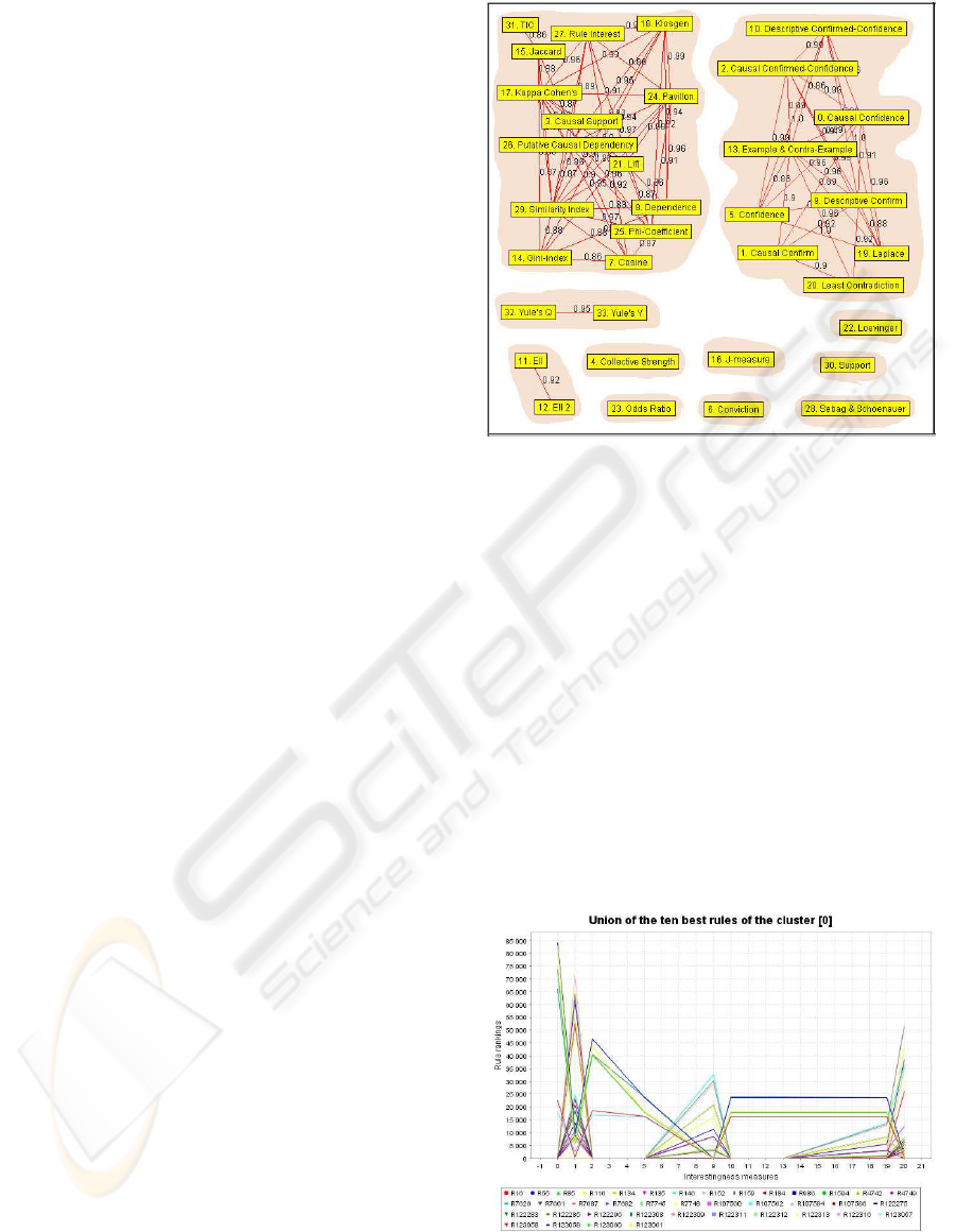
edge is given from the strongly positive correlation

value (see Fig. 4).

Based on the strongly positive correlation and con-

structed with the weighted graph, we have found

eleven positively correlated clusters (Fig. 4):

- (C0) Least Contradiction, Causal Conﬁrm,

Laplace, Conﬁdence, Descriptive Conﬁrm, Exam-

ple & Contra-Example, Causal Conﬁdence, Causal

Conﬁrmed-Conﬁdence, Descriptive Conﬁrmed-

Conﬁdence. These measures have formed the

cluster because most of these measures are issued

from conﬁdence measure.

- (C1) Cosine, Gini-index, Phi-Coefﬁcient, Similar-

ity Index, Dependence, Lift, Putative Causal De-

pendency, Causal Support, Kappa Cohen’s, Pavil-

lon, Jaccard, Rule Interest, TIC, Klosgen.

- (C2) Yule’s Q and Yule’s Y are the measures

that form a cluster, the same result as Tan (Tan

et al., 2004) with the effect of the second property,

row/column scaling invariance. This conclusion is

not very surprising because of our demonstration

in Section 3 these measures are functionally depen-

dent (See Appendix B for more details).

- (C3) EII and EII 2, the two entropic versions of the

measure Intensity of Implication. These two mea-

sures are issued from the change of one parame-

ter in their formula (α = 1 or α = 2) (Blanchard

et al., 2003), so this cluster is naturally and strongly

within-related.

- (C4..C10) Seven clusters with a single measure:

Collective Strength, Odds Ratio, J-measure, Con-

viction, Loevinger, Support, and Sebag & Schoe-

nauer, which are not strongly correlated to other

ones.

5.4 Best rules

5.4.1 Intersection of the ten best rules

We choose the ten best rules of each positive cluster

and give the user an overview of their intersection.

The rank of each rule is used to validate the result.

The Y-axis holds the rank of the rule for the corre-

sponding measure. Each rule is represented with par-

allel coordinates among interestingness measure val-

ues (see Fig. 5). We can see the intersection in a

horizontal line and if we obtain many rules having the

same rank value so we will print these rules with only

one line. If the user want to capture a small group

of the best rules for making their decision, he/she can

use these rules for their ﬁrst choice.

Figure 4: Weighted graph from Mushroom data set.

5.4.2 Union of the ten best rules

With the same technique as above, we introduce the

union of the ten best rules in each cluster, in order to

give the user a more speciﬁc view in the cluster . The

measures have the set of highest ranks (more interest-

ing) rely on the low value of the Y-axis. With the con-

centration lines on low rank values, we can capture

3 measures: Conﬁdence(5), Descriptive Conﬁrmed-

Conﬁdence (10), and Example Contra-Example (13)

that are suitable for all of the best rules in this cluster

(see Fig. 5).

Figure 5: Within-cluster union of one positive cluster from

Mushroom data set.

CLUSTERING INTERESTINGNESS MEASURES WITH POSITIVE CORREALTION

251

5.5 Clusters in relation to a selected

cluster

With the same technique used in the Section 5.4, we

introduce the two following views :

5.5.1 Union of all the clusters in relation to the

current cluster

Based on the ten best rules in the current cluster, we

draw the parallel coordinates of each rule on other

clusters. The user can see the zone that is the most

interesting with the highest value. The effect of the

ten best rules on the other clusters gives the user a

general sampling of the entire cluster. With the union

approach, many best rules may be presented and com-

pared.

5.5.2 Intersection of all the clusters in relation to

the current cluster

By decreasing the quantity of best rules in one clus-

ter, we will observe the rank distribution. The inter-

section is less interesting than the union because we

generally do not have any interesting zone. Using the

intersection in relation to the current cluster is impor-

tant when the user just ﬁnds a small set of interesting

and close rules.

6 CONCLUSION

This work has led to the implementation of a tool em-

bedding more than 8000 lines of Java codes for the

analysis of data set characteristics, quality measure

sensitivity, correlations, clustering and ranking.

We have found and identiﬁed eleven clusters from

all the quality measures studied on the Mushroom

data set. We have also proposed a way to study the

ten best rules of each cluster, the union and intersec-

tion of the ten best rules of all the cluster in relation to

the current cluster. The union of the ten best rules for

all the clusters is also presented for the user’s choice.

For the ﬁrst presentation of our results, we just use

thirty four measures for implementation.

Our future research will focus on improving the

clustering of measures: (1) in designing a better sim-

ilarity measure than the linear correlation, (2) in se-

lecting the best representative measure in a cluster.

REFERENCES

Agrawal, R., Imielinski, T., and Swami, A. (1993). Mining

association rules between sets of items in large data-

bases. In Proceedings of 1993 ACM-SIGMOD Inter-

national Conference on Management of Data.

Agrawal, R. and Srikant, R. (1994). Fast algorithms for

mining association rules. In Proceedings of the 20th

VLDB Conference.

Bayardo, J. and Agrawal, R. (1999). Mining the most in-

terestingness rules. In Proceedings of the Fifth ACM

SIGKDD International Confeference On Knowledge

Discovery and Data Mining.

Blake, C. and Merz, C. (1998). UCI Repos-

itory of machine learning databases,

http://www.ics.uci.edu/∼mlearn/MLRepository.html.

University of California, Irvine, Dept. of Information

and Computer Sciences.

Blanchard, J., Kuntz, P., Guillet, F., and Gras, R. (2003).

Implication intensity: from the basic statistical deﬁn-

ition to the entropic version. In Statistical Data Min-

ing and Knowledge Discovery. Chapman & Hall, CRC

Press.

Brin, S., Motwani, R., and Silverstein, C. (1997). Beyond

market baskets: Generalizing association rules to cor-

relation. In Proceedings of ACM SIGMOD Confer-

ence.

Freitas, A. (1999). On rule interestingness measures. In

Knowledge-Based Systems, 12(5-6).

Gavrilov, M., Anguelov, D., Indyk, P., and Motwani, R.

(2000). Mining the stock market: which measure is

best? In Proceedings of the Sixth International Con-

ference on Knowledge Discovery and Data Mining.

Gras, R. (1996). L’implication statistique - Nouvelle

ethode exploratoire de donn

ees. La pens

ee sauvage

edition.

Hilderman, R. and Hamilton, H. (2001). Knowledge Dis-

covery and Measures of Interestingness. Kluwer Aca-

demic Publishers.

Klemettinen, M., Mannila, H., Ronkainen, P., Toivonen, H.,

and Verkano, A. I. (1994). Finding interesting rules

from larges sets of discovered association rules. In the

Third International Conference on Information and

Knowledge Management. ACM Press.

Kononenco, I. (1995). On biases in estimating multi-valued

attributes. In Proceedings of the Fourteenth Interna-

tional Joint Conference on Artiﬁcial Intelligence (IJ-

CAI’95).

Liu, B., Hsu, W., Mun, L., and Lee, H. (1999). Finding

interestingness patterns using user expectations. In

IEEE Transactions on Knowledge and Data Mining

11(1999).

Padmanabhan, B. and Tuzhilin, A. (1998). A belief-

driven method for discovering unexpected patterns.

In Proceedings of the 4th international conference on

Knowledge Discovery and Data Mining.

Piatetsky-Shapiro, G. (1991). Discovery, analysis and pre-

sentation of strong rules. In Knowledge Discovery in

Databases. MIT Press.

Saporta, G. (1990). Probabilit

es, Analyse des Donn

ees et

Statistique. Editions Technip, Paris.

ICEIS 2005 - ARTIFICIAL INTELLIGENCE AND DECISION SUPPORT SYSTEMS

252

Silberschartz, A. and Tuzhilin, A. (1996). What makes pat-

terns interesting in knowledge discovery systems. In

IEEE Transaction on Knowledge and Data Engineer-

ing (Vol. 8, No. 9).

Tan, P., Kumar, V., and Srivastava, J. (2004). Selecting the

right objective measure for association analysis. In

Information Systems 29(4).

Appendix B. Relation between measures

◦

Formulae

0 Laplace =

Conf idence×(n×Support+1)

n×Support+2×Con f idence

1 RuleInterest =

S upport

Conf idence

× P avillon

2 Lift =

Conf idence

Conf idence−P avillon

3 W ang =

S upport

Conf idence

× (Confidence − α)

4 Gray&Orlowska =

(Lift

− 1) × (Support − RuleInterest)

5 J − measure = Support × log

(Lift) + (Support

−DescriptiveConf irm) × log 2(

Conviction

)

6 J − measurevariant = Support × log

(Lift)

7 Jaccard =

S upport

Conf idence

+Conf idence−P avillon−Support

8 Loevinger = 1 −

Conviction

9 Consine =

S upport

√

S upport−RuleInterest

10 CausalConf irm = CausalSupport − 2 × Support+

2 × Descriptiv eConf irm

11 CausalConf irmed − Conf idence =

DescriptiveConf irmedConf idence − Conf idence+

CausalConf idence

12 Consine

= Lif t × Support

13 RuleInterestvariant = |RuleInterest|

14 T auxDeLiaison = Lift − 1

15 Y ule

′

sQ =

OddsRatio−1

OddsRatio+1

16 Y ule

′

sY =

√

OddsRatio−1

√

OddsRatio+1

17 Example&Contra − Example =

DescriptiveConf irm

Conf idence−P avillon

18 LeastContradiction =

DescriptiveConf irm

19 Klosgen =

√

Support × P avillon

20 Sebag&Schoenauer =

S upport

S upport−DescriptiveConf irm

Appendix A. Quality measures

◦

Interestingness Measure f(n, n

, n

)

0 Causal Conﬁdence 1 −

(

1 Causal Conﬁrm

−4n

2 Causal Conﬁrmed-Conﬁdence 1 −

(

3 Causal Support

−2n

4 Collective Strength

−n

)(n

−n

)(n

)

)(n

−n

+2n

)

5 Conﬁdence 1 −

6 Conviction

7 Cosine

−n

√

8 Dependence |

−

9 Descriptive Conﬁrm

−2n

10 Descriptive Conﬁrmed-Conﬁdence 1 − 2

11 EII (α = 1) ϕ × I

2α

12 EII (α = 2) ϕ × I

2α

13 Example & Contra-Example 1 −

−n

14 Gini-index

−n

)

−n

)

+(n

−n

)

−

15 Jaccard

−n

16 J-measure

−n

log

n(n

−n

)

log

17 Kappa Cohen’s

2(n

−nn

)

18 Klosgen

−n

(

−

)

19 Laplace

+1−n

20 Least Contradiction

−2n

21 Lift

n(n

−n

)

22 Loevinger 1 −

23 Odds Ratio

−n

)(n

−n

)

−n

)

24 Pavillon

−

25 Phi-Coefﬁcient

−nn

√

26 Putative Causal Dependency

−3n

− (

27 Rule Interest

(

− n

)

28 Sebag & Schoenauer 1 −

−n

29 Similarity Index

−n

−

30 Support

−n

31 TIC T I(a → b) × T I(b → a)

32 Yule’s Q

−nn

+(n

−n

−2n

+2n

33 Yule’s Y

−n

)(n

−n

)−

−n

)

−n

)(n

−n

)

CLUSTERING INTERESTINGNESS MEASURES WITH POSITIVE CORREALTION

253